
The SUMIF function in Excel is an effective way to total values that meet specific conditions. But if you only want to match part of the text like entries that contain, start with, or end with a certain word, then wildcards come in handy.
In this article, you’ll learn how to perform a SUMIF partial match at specific or non-specific positions using the asterisk (*) wildcard. You’ll also see how to combine it with SUMIFS for multiple criteria using a real dataset. Let’s get started.
➤ Type the following formula:
=SUMIF(A2:A11,”*apple*”,C2:C11)
➤ Press Enter, and Excel will display the total sales for all “apple” related products.
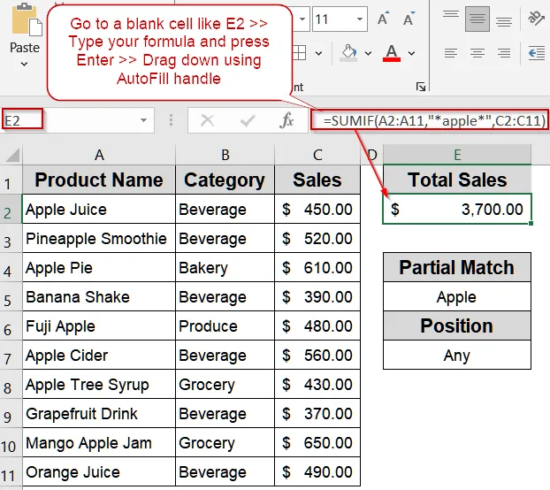
Detect Text Anywhere in a Cell with Direct Reference Using Wildcard
When dealing with datasets where keywords can appear in multiple positions such as in beginning, middle, or end of a product name, capturing all relevant entries is crucial. Using a wildcard allows you to sum all matching values, ensuring nothing is missed. We’ll use the following dataset with sales information for different products:
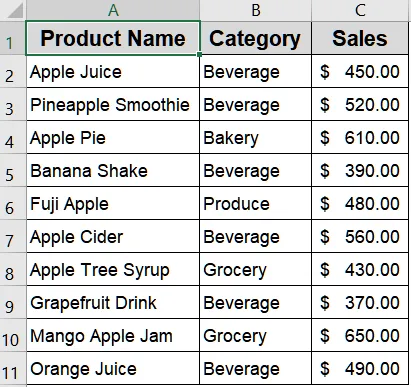
➤ Select a blank cell where you want the result to appear.
➤ Type the following formula:
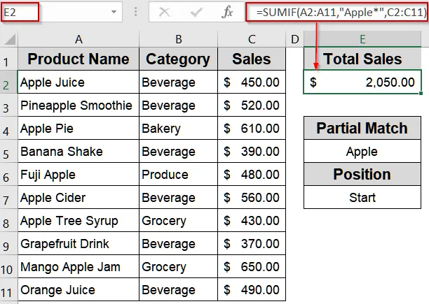
=SUMIF(A2:A11,"*apple*",C2:C11)➤ Press Enter, and Excel will display the total sales for all “apple” related products.
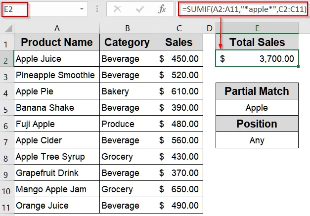
Identify Text Starting with a Specific Word
In situations where items follow a naming convention or you only want to include entries beginning with a specific keyword, filtering by the starting text is essential. This helps focus your totals on precisely the items that match your criteria.
➤ Select an empty cell.
➤ Type the following formula:
=SUMIF(A2:A11,"Apple*",C2:C11)➤ Hit Enter to display the total for all products that start with “Apple.”
Target Text Ending with a Specific Word
Sometimes keywords appear at the end of text, such as suffixes, regional codes, or product variations. Summing values based on the ending ensures you capture only the intended entries without accidentally including unrelated items.
➤ Click on a blank cell.
➤ Type the following formula:
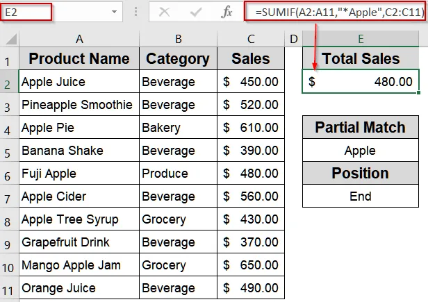
=SUMIF(A2:A11,"*Apple",C2:C11)➤ Press Enter to get your result.
Combine Multiple Conditions Using SUMIFS Function
When your analysis requires more than one condition, this method is highly effective. SUMIFS function allows you to sum values while applying multiple criteria simultaneously, such as filtering by product name and category at the same time. It’s useful for more complex datasets where a single condition isn’t sufficient to capture the data you need.
➤ Choose a cell for the result.
➤ Type the following formula:
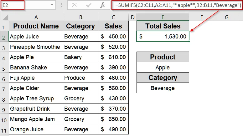
=SUMIFS(C2:C11,A2:A11,"*apple*",B2:B11,"Beverage")➤ Press Enter, and you’ll get total sales for all apple beverages.
Add Partial Matches Using Cell Reference
Instead of referencing the keyword inside the formula, you can assign the keyword you are looking for to a specific cell to make it the calculation dynamic. It’s perfect for situations where you frequently change the keyword or need a more interactive spreadsheet. This approach reduces errors and makes updating your analysis quick and easy.
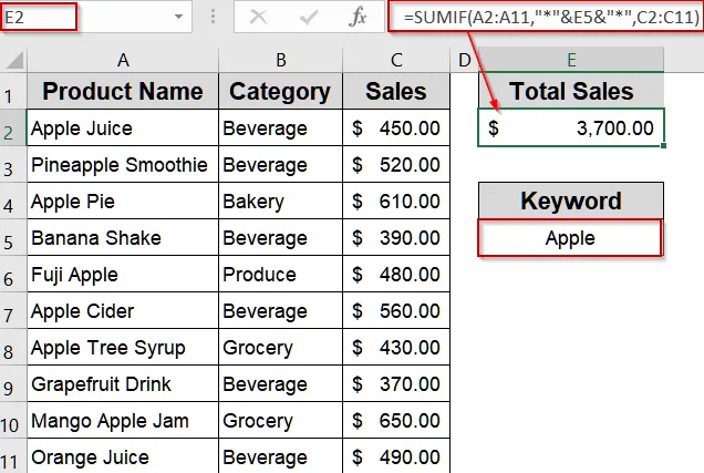
➤ Type your keyword (e.g., apple) in cell E5.
➤ In another cell, type the following formula:
=SUMIF(A2:A11,"*"&E5&"*",C2:C11)➤ Press Enter to get your total automatically.
Include Asterisk as a Literal Character in SUMIF Formula
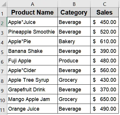
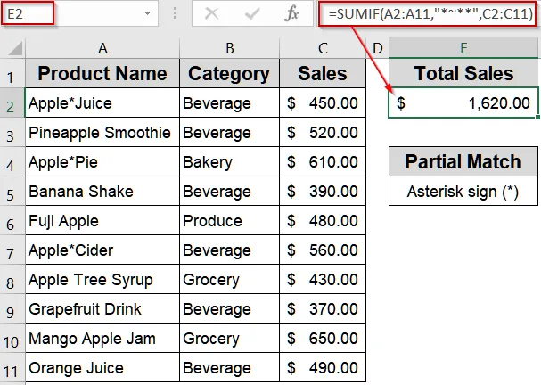
Sometimes your dataset contains an actual asterisk (*) that is part of the product name or description. Normally, Excel treats an asterisk as a wildcard, but this method shows how to sum values for items containing a literal asterisk. It’s essential for accurate calculations when your data uses special characters in names or codes.
We’ll use the following modified dataset:
➤ Select an empty cell.
➤ Type the following formula:
=SUMIF(A2:A11,"*~**",C2:C11)➤ Press Enter to calculate the total.
Replace Keywords Before Summing Using Find and Replace
Data inconsistencies, like “Apple”, “Apples” or “Apple-” can affect totals if left uncorrected. Standardizing keywords using Find and Replace ensures uniform text, improving the accuracy of your SUMIF function calculations. This method focuses on cleaning and standardizing your dataset before performing any calculations. We’ll use the following modified dataset:
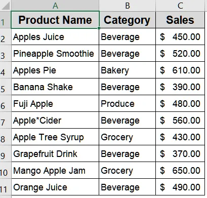
➤ Press Ctrl + H to open the Find and Replace dialog box.
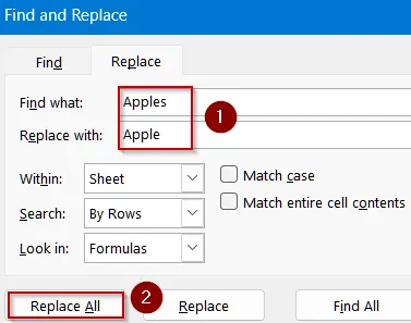
➤ In “Find what”, type the unwanted variation (e.g., “Apples”).
➤ In “Replace with”, type the standardized word (e.g., “Apple”).
➤ Click Replace All to clean the dataset.
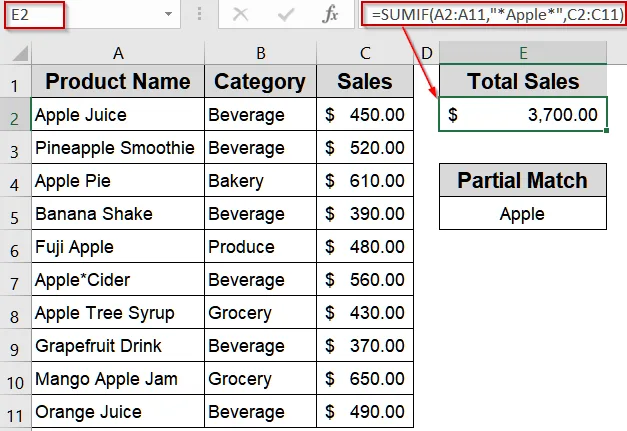
➤ Now apply the following formula to total sales:
=SUMIF(A2:A11,"*Apple*",C2:C11)➤ Press Enter for output.
Downloadable Resources
Get our practice workbook or necessary files that we have worked with to prepare this article.
SUMIF with Partial Match.xlsx
Practice Workbook · Excel (.xlsx)
Frequently Asked Questions
What does the asterisk (*) mean in a SUMIF partial match?
The asterisk acts as a wildcard character that represents any number of characters. It allows SUMIF function to match text that contains, starts with, or ends with a specific keyword easily in Excel.
Can I use SUMIF partial match for case-sensitive data?
No, the SUMIF function in Excel is not case-sensitive. It treats “Apple” and “apple” as the same. If you need a case-sensitive match, you must use advanced formulas like SUMPRODUCT function.
Why is my SUMIF partial match returning incorrect results?
Incorrect results often occur when your ranges are mismatched or contain extra spaces. Always ensure the criteria range and sum range are equal in size and clean the data using TRIM function if necessary.
How do wildcards differ in SUMIF and SUMIFS functions?
Wildcards work the same in both functions. However, SUMIFS lets you apply multiple conditions, such as matching text partially in one column while filtering by category or region in another column.
Can I combine cell references and partial matches together?
Yes, you can. Concatenate the reference with wildcards like =SUMIF(A2:A11,”*”&E2&”*”,C2:C11). This setup automatically adjusts the criteria when you change the keyword stored in the referenced cell.
Wrapping Up
In this tutorial, you learned how to use SUMIF with partial matches in different ways whether you’re checking if a word appears anywhere, starts, or ends in a text. By combining wildcards with SUMIF and SUMIFS functions, you can summarize data precisely without manually filtering rows. Feel free to download the practice file and share your feedback.