
In academic and professional contexts, we need to calculate the percentage of marks. It is one of the most common Excel tasks. Teachers, school administrators, and even students frequently need to convert raw scores into percentages for evaluation. One of the most widely used formulas to calculate percentage in a marksheet is:
= (Obtained Marks / Total Marks) * 100
This simple formula converts any student’s marks into a percentage. However, Excel also has some alternative methods to calculate percentage.
To use percentage formula in Excel for marksheet, follow these simple steps:
➤ Calculate total marks using =SUM(B2:D2)
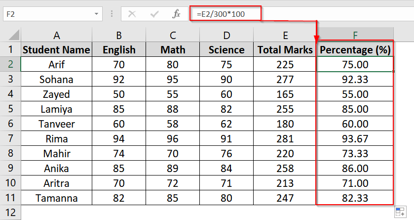
➤ Use the formula =E2/300*100 to get the percentage.
➤ Format the cell using the Percent Style (%) button in Excel.
This article will show how to use the percentage formula in excel for marksheets using different formulas (like Baic Formula, Percent Style) and functions like SUM.
Using Sum & Percentage Formulas to Calculate Percentage in Excel
When student marks are distributed across multiple columns representing different subjects we use Sum Function. By summing the marks and dividing by the full mark total, you can quickly calculate the percentages for each student. It’s commonly used in academic marksheets where subject scores.
We have a dataset where three subjects are listed per student. We will use the SUM function to calculate the total marks obtained across all subjects and then divided by the total possible marks (300) to get the percentage.
Steps:
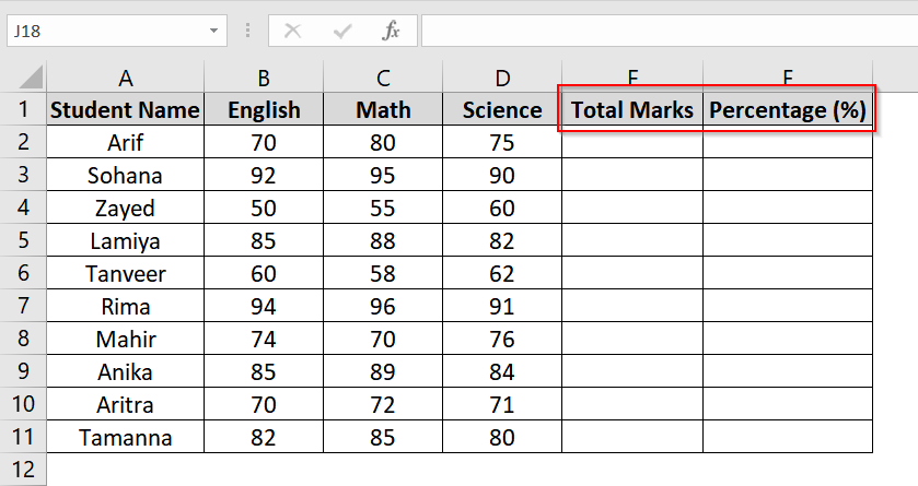
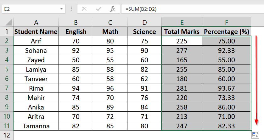
➤ Open your Excel worksheet. Label the Column E (next to Science) header as Total Marks and Column F as Percentage (%)
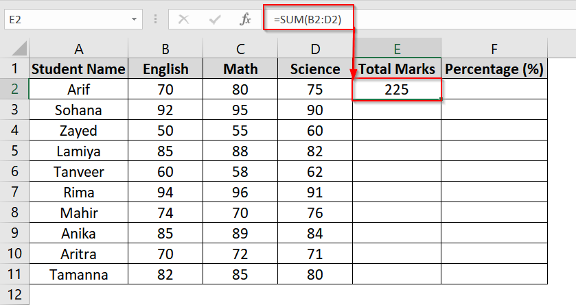
➤ Click on cell E2 and enter the formula:
=SUM(B2:D2)
This will calculate the total marks for the first student.
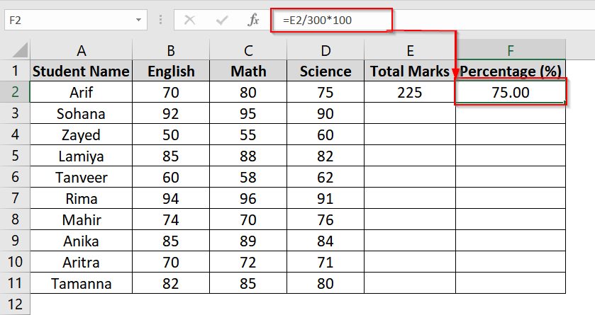
➤ In cell F2, type the formula and press enter:
=E2/300*100
This divides the total marks by the full mark (300) and multiplies by 100 to get the percentage. You’ll get the percentage for the first student. Format the result with the Percent Style if preferred.
➤ Drag the fill handle down in both Columns G and H to apply the formulas to other students.
Note:
➥ Ensure all students are being assessed out of the same total marks.
➥ Replace 300 in the formula with actual full marks if it differs.
➥ To avoid decimals, you can wrap the formula in ROUND like =ROUND(E2/300*100,2).
Applying Basic Percentage Formula for Marksheet in Excel
This method can calculate the percentage of marks obtained by a student in an exam. It is used when you know both the marks obtained and the total marks for each student. This formula is needed for standard mark sheets that are used in schools or colleges where results need to be shown in percentage format.
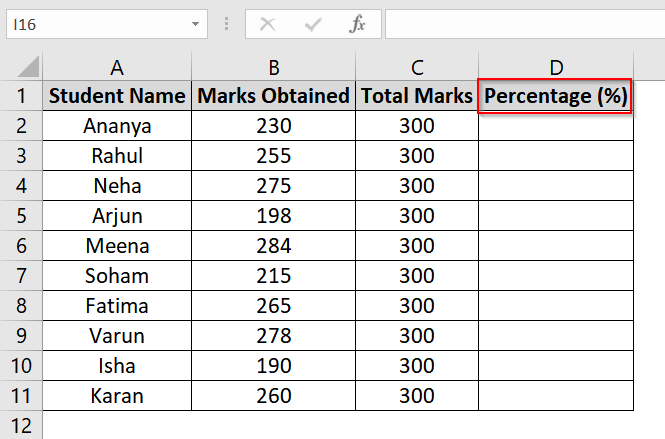
We have a dataset where the student names in Column A, marks obtained in Column B, and total marks in Column C. In Column D we want the percentage to be displayed.
Steps:
➤ Open your Excel sheet or dataset where you want to apply, calculate the percentage for the marksheet or open up our demo worksheet after downloading it. Rename the D1 cell as “Percentage (%)”
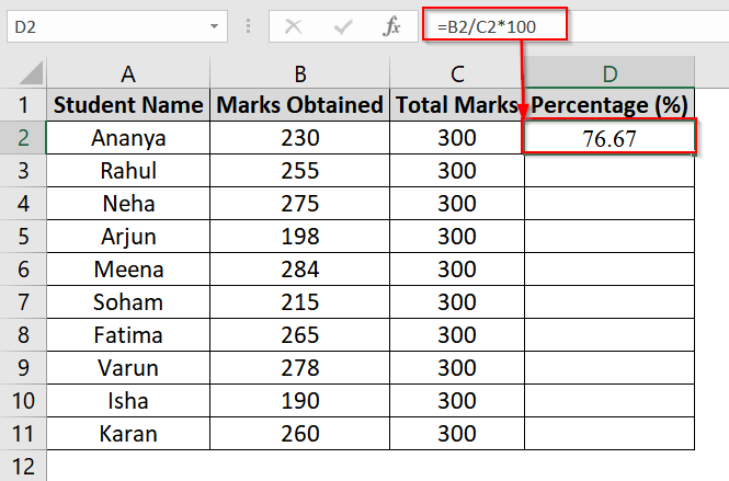
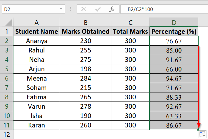
➤ In cell D2 , type the formula:
=B2/C2*100
➤ Press Enter. This will calculate the percentage of obtained mark for the first student.
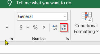
➤ (Optional) Format the result as a percentage with 2 decimal places. To do that, go to the Home tab → In the Number group, click the decrease decimal places.
➤ Use the Fill Handle (small square at the bottom-right corner of the selected cell) to drag the formula down for all rows.
Note:
Ensure all rows in the “Total Marks” column have values to avoid division by zero.
Using Percent Style with Formula for Marksheet in Excel
Percent Style can calculate student percentages using a basic division formula and Excel’s Percent Style formatting. It is best when you want clean, readable percentage values with automatic formatting. Here we will calculate Percentage of students obtained a mark using obtained mark and total mark.
Steps:
➤ Open your Excel worksheet. We have taken a dataset where
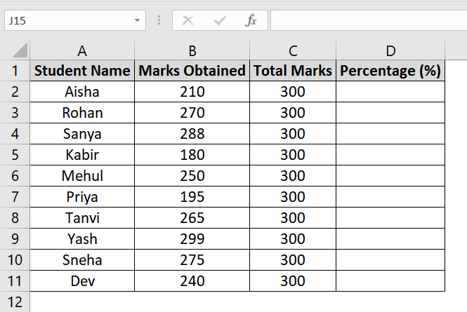
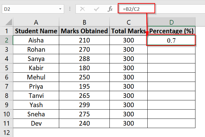
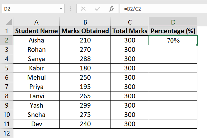
➤ Click on cell D2 (next to the first student) to insert the percentage formula. Type the formula and click enter.
=B2/C2
This gives a decimal value (e.g., 0.7 for 70%).
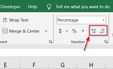
➤ While D2 is selected, go to the Home tab → Number group → click on Percent Style (%).
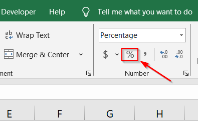
➤ This will convert 0.7 to 70%.
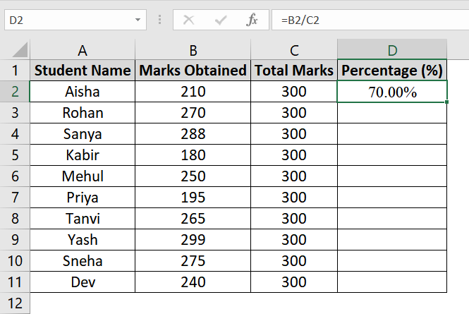
➤ To show two decimal places, click on Increase Decimal (found next to Percent Style).
➤ It looks like this-
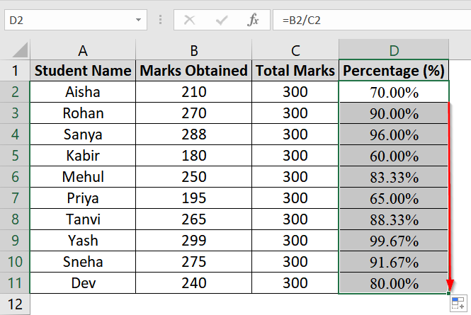
➤ Use the Fill Handle from the corner of D2 to drag the formula down to all rows.
Note:
➥ Percent Style automatically multiplies decimal results by 100 and adds a percent sign (%).
➥ Avoid typing *100 when using Percent Style, or you’ll get incorrect results (e.g., 7000% instead of 70%).
Calculate Obtained Marks from Percentage and Total Marks in Excel
This method is used when you know the percentage scored and the maximum total marks for a subject or exam, and you want to calculate how many marks a student actually obtained. This is helpful for reversed scoring systems or grade-based mark retrieval in academic datasets.
We have taken a dataset where we have student names in Column A, their scoring percentage in Column B, and total marks in Column C. We will have the calculated mark in column D named as “Obtained Mark”
Steps:
➤ Open your dataset where you want to perform the percentage based calculation.
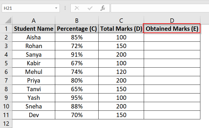
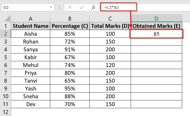
➤ Select the first empty cell in Column E (e.g., E2) beside the first row of student data. Type the formula and press enter:
=C2*B2
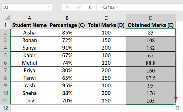
This multiplies the total marks by the percentage to get the obtained marks.
➤ Drag the fill handle down to fill the formula for all students.
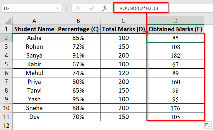
➤ (Optional): Round off the results if you want whole number marks only using:
=ROUND(D5*C5, 0)
Note:
➥ The percentage must be entered correctly as a percentage, not a whole number. For example, 85% should not be entered as “85” but as “0.85” or use Excel’s percent format.
➥ Total marks must be numeric and non-empty.
Frequently Asked Questions (FAQs)
What is the formula of percentage in Excel?
Use =obtained_marks / total_marks, then apply Percent Style.
How to calculate average in marksheet?
Use =AVERAGE(B2:E2) where B2 to E2 are the subject marks.
What is a percentage formula?
Percentage formula is a method to convert raw scores to percentages, usually by dividing obtained marks by total marks and multiplying by 100.
How do I remove percentage in Excel?
Select the cells, right-click, choose “Format Cells“, and change it from “Percentage” to “General” or “Number“.
Concluding Words
In this guide, we used the Percent Style Method , Basic Percentage method to calculate the percentage in an Excel marksheet. We have combined simple functions like =SUM and division formula with percentage formatting. If you are calculating class performance or analyzing results, these described methods can save time and reduce errors. Also, if you have any queries let us know.