With a randomized list of names, you can do team grouping, customer research, surveys, and more. Although Excel has no direct built-in functions or add-ins to randomize names, it has the RAND and RANDBETWEEN functions to generate random numbers.
So, we can use them to assign random numbers to each cell containing the names. After that, combining the INDEX and ROWS functions will give us the values from those randomly shuffled cells.
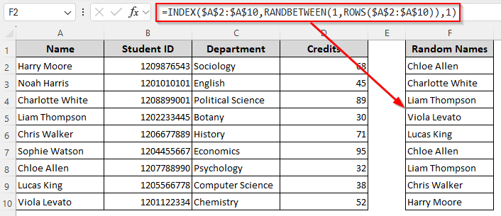
To randomize a list of names with the INDEX, RANDBETWEEN, and ROWS functions:
➤ Select a blank cell in a column where you want to enter the shuffled names and type the following formula:
=INDEX($A$2:$A$10,RANDBETWEEN(1,ROWS($A$2:$A$10)),1)
➤ The names we want to randomize are in the cells $A$2:$A$10. Change the range as required.
➤ Click Enter and the formula will give one random name from the list. Drag the formula down to fill the column with the entire list of randomized names.
In this article, we’ll cover all the ways of randomizing a list of names with Power Query, VBA coding, and functions like RAND, RANDBETWEEN, INDEX, SORTBY, CHOOSE, etc.
Randomizing Names with RAND/RANDBETWEEN Function & Sorting
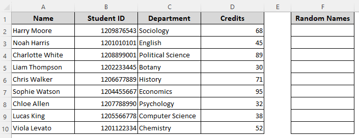
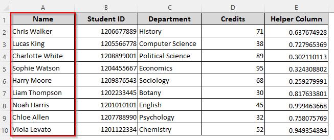
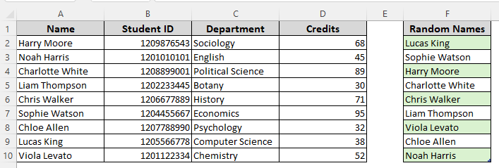
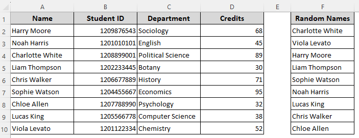
To demonstrate each method, we have a dataset with columns for student names, IDs, departments, and more related info. Our goal is to randomize the student names from column A and put them in column F.
With the RAND function, you can assign random numbers to each row of your selection. The RANDBETWEEN function does the same, except that it only assigns integers instead of fractions. While using this method, we’ll assign a random number to each row and sort it with our original dataset.
So, we get randomly sorted values in our source data. This method is preferable when you only have a name column to shuffle. Avoid this method if you have multiple related columns and you don’t want any changes in the original data source. Below are the steps:
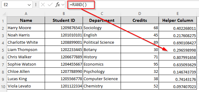
➤ Create a helper column and enter any of the following formulas in its first cell:
=RAND()
Or,
=RANDBETWEEN(1,9)
➤ We selected the numbers 1 to 9 as we have 9 rows of names. Change the numbers according to your dataset.
➤ Press Enter and drag the formula down to the remaining cells using the fill handle (+ sign on the cell’s bottom corner).
➤ As Excel returns a number for each row, select your entire dataset and go to the Data tab. Click on Sort.
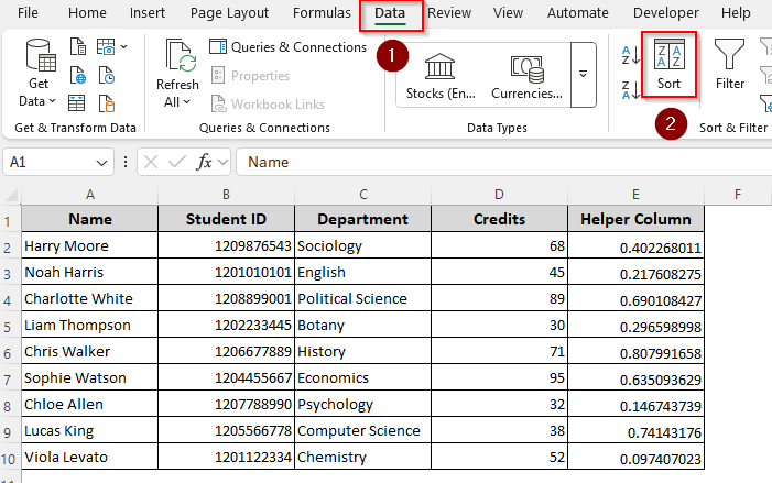
➤ When the Sort window opens, click on the Sort By drop-down and select the Helper Column from the list.
➤ From the Order drop-down, choose Largest to Smallest.
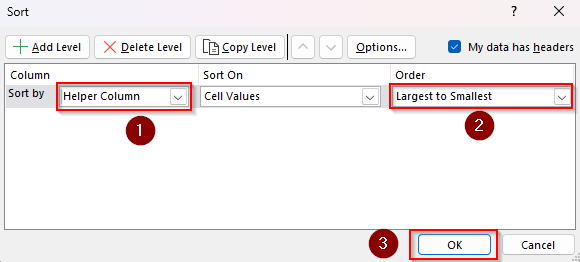
➤ Press Ok to randomize your entire dataset, including the listed names. Once done, you can delete the helper column.
Randomly Select Names Using the CHOOSE and RANDBETWEEN Functions
For smaller datasets, you can use the CHOOSE and RANDBETWEEN functions to input each cell reference containing the names and shuffle them. You need to manually enter each cell reference in the formula, so it’s not a convenient method for large datasets. Also, it returns duplicate names.
As the RANDBETWEEN function returns a random whole number for each cell, the CHOOSE function uses that number to pick a random name from the list. Here’s how to combine them:
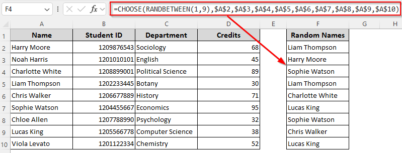
➤ In the output cell, enter the following formula:
=CHOOSE(RANDBETWEEN(1,9),$A$2,$A$3,$A$4,$A$5,$A$6,$A$7,$A$8,$A$9,$A$10)
➤ As we have 9 rows with names, we assigned random numbers between 1 to 9 using the RANDBETWEEN function. Change it and the cell references according to your dataset. You can also enter the names directly instead of the cell references.
➤ Click Enter and drag the formula down to fill the remaining cells with random names from column A.
Note:
All the functions for randomizing data such as RAND and RANDBETWEEN change the return values every time you make any changes in your worksheet. To freeze the result, first, copy the cells with shuffled names. Click on the Home tab >> Paste >> Paste Special >> Values >> Ok.
Randomize Names Using the INDEX, RANDBETWEEN, and ROWS Functions
When the RANDBETWEEN and ROWS/COUNTA functions assign random numbers for the counted rows, the INDEX function extracts the values from those rows. Combining these functions allows you to randomize the names in a specific range. This method might also return duplicates. Follow the steps below:
➤ Select a cell to put the first returned random name and enter any of the formulas given below:
For a Known Number of Rows
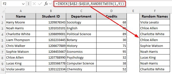
➤ If you know how many cells/rows you’re working with, type this formula:
=INDEX($A$2:$A$10,RANDBETWEEN(1,9))
➤ We entered (1, 9) as our range has 9 names. Change the numbers and the data range $A$2:$A$10 according to your dataset.
➤ Press Enter and drag the formula down.
For an Unknown Number of Rows without Blanks
When you don’t know how many rows of names you have, enter this formula instead:
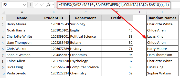
=INDEX($A$2:$A$10,RANDBETWEEN(1,ROWS($A$2:$A$10)),1)
➤ Change the cell range as needed. Press Enter and drag the formula down.

For an Unknown Number of Rows with or without Blanks
With blank cells in your range, the formula above can return errors. So, use this formula instead:
=INDEX($A$2:$A$10,RANDBETWEEN(1,COUNTA($A$2:$A$10)),1)
➤ Replace the cell range if required and press Enter. Use the fill handle to drag down and randomize the entire list.
Dynamic Array Sampling of Random Names (No Duplicates)
If you have Excel 365 or 2021+, you can instantly shuffle a list of names using the SORTBY, RANDARRAY, and ROWS/COUNTA functions. As we combine RANDARRAY and ROWS/COUNTA, they create a random number for each row of your data range.
The SORTBY function then shuffles all names based on those random numbers. Let’s get to the steps:
➤ In the output cell where you want the randomized list, insert any of the formulas given below:
For Datasets with No Blank Cells
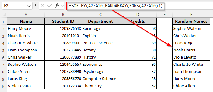
➤ Use the following formula and click Enter. This spills a randomly sorted version of your list.
=SORTBY(A2:A10,RANDARRAY(ROWS(A2:A10)))
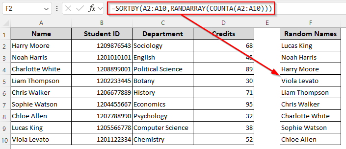
For Datasets with Non-Blank and Blank Cells
➤ Type the following formula and click Enter:
=SORTBY(A2:A10,RANDARRAY(COUNTA(A2:A10)))
Randomly Sort the Names in a List Using Power Query
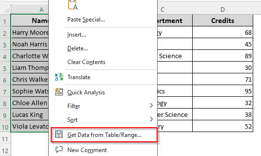
For complex datasets or an Excel table, using the Power Query tool is more suitable for shuffling a list of names. Here’s how to use it:
➤ Select the cell range containing the names and right-click on your mouse. Select Get Data from Table/Range from the menu.
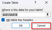
➤ If Excel prompts you to turn your data into a table, press Cancel.
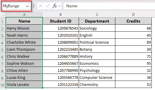
➤ Go to the name bar and give a name to your dataset. Click Enter, right-click, and choose Get Data from Table/Range again.
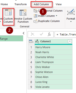
➤ In the Power Query Editor, click on the Add Column tab and select Custom Column.
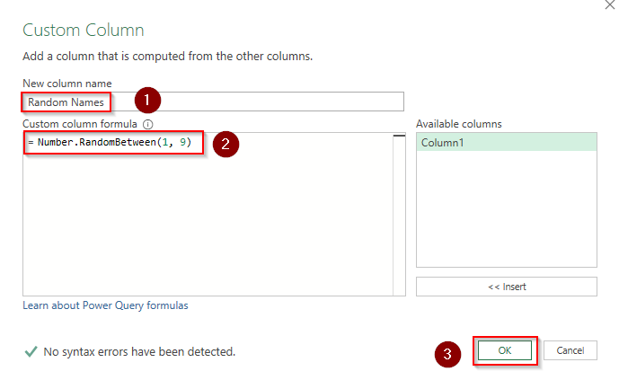
➤ Now, give the new column a name and enter this formula in the Custom Column Formula editor:
= Number.RandomBetween(1, 9)
➤ Change (1, 9) according to the row numbers of your dataset.
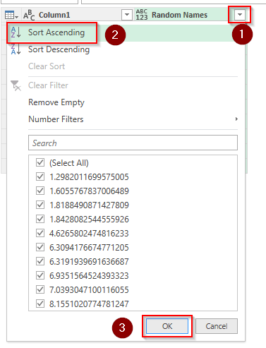
➤ As each row gets a random number, select your entire dataset and click on the Filter drop-down on the new custom column heading.
➤ Choose Sort Ascending from the menu and click Ok.
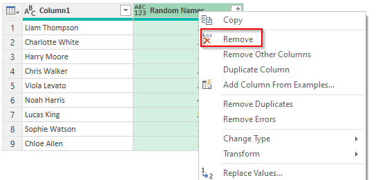
➤ Once the names are sorted, you can highlight the added column, right-click on it, and click on Remove.
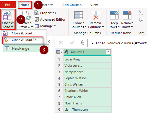
➤ Now, go to the Home tab, click on the Close & Load drop-down >> Close & Load To.
➤ Select a location to put the shuffled list and press Ok.
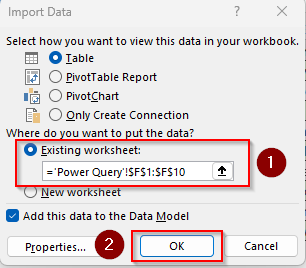
➤ Here’s the final result for our dataset:
Shuffle Names with a Custom VBA Macro
With the Developer tool, you can create a VBA macro that randomizes the data you select. For this, simply follow the steps given below:
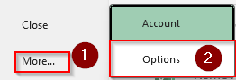
➤ To add the Developer tab, go to the File tab >> More >> Options.
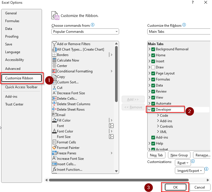
➤ Click on Customize Ribbon and check the Developer tab. Press Ok.
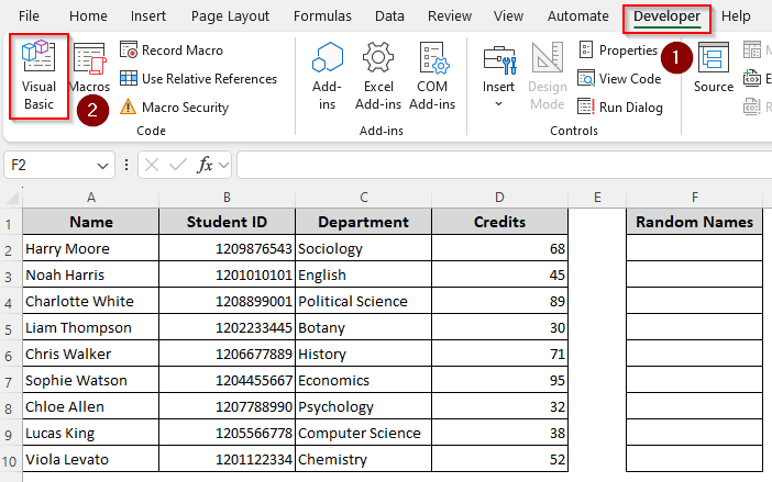
➤ Now, click on the Developer tab and choose Visual Basic.
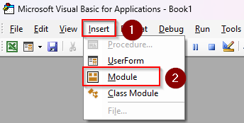
➤ In the VBA Editor, press Insert and choose Module.
➤ Paste the following code in the blank field:
Sub RandomizeNameList()
Dim nameRange As Range
Dim outputCell As Range
Dim tempList() As Variant
Dim shuffledList() As Variant
Dim i As Long, j As Long
Dim temp As Variant
' Prompt user to select the list of names
On Error Resume Next
Set nameRange = Application.InputBox("Select the range containing the names to randomize:", "Select Name Range", Type:=8)
If nameRange Is Nothing Then Exit Sub
' Prompt user to select the output cell
Set outputCell = Application.InputBox("Select the cell where the first randomized name should go:", "Select Output Cell", Type:=8)
If outputCell Is Nothing Then Exit Sub
On Error GoTo 0
' Load the names into an array
tempList = Application.Transpose(nameRange.Value)
ReDim shuffledList(1 To UBound(tempList))
' Shuffle the array using Fisher-Yates algorithm
shuffledList = tempList
For i = UBound(shuffledList) To 2 Step -1
j = Int(Rnd() ➤ i) + 1
temp = shuffledList(i)
shuffledList(i) = shuffledList(j)
shuffledList(j) = temp
Next i
' Output the shuffled names starting from the selected cell
For i = 1 To UBound(shuffledList)
outputCell.Offset(i - 1, 0).Value = shuffledList(i)
Next i
MsgBox "Names have been randomized!", vbInformation
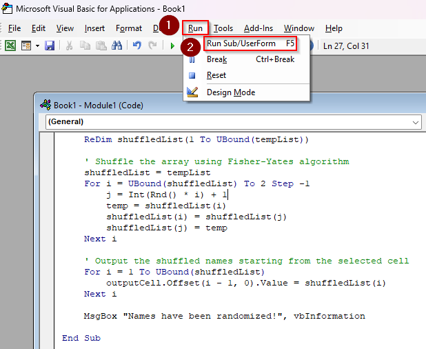
End Sub➤ Press F5 to run the code or click on the Run tab >> Run Sub/UserForm.
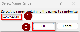
➤ As Excel prompts you to select the name range to shuffle, go to the Excel tab and highlight the cells. Click Ok.
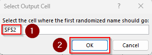
➤ After that, manually enter or highlight the cell reference where you want to put the first random name. Press Ok.
➤ Excel will now return the randomized names in your selected location.
Frequently Asked Questions
How to recalculate a randomized list in Excel?
If you use formulas like RAND, RANDBETWEEN, or RANDARRAY, Excel recalculates them automatically when you edit a cell. For other functions, press F9 to recalculate the entire workbook. To recalculate the active sheet only, press SHIFT + F9 .
How to randomize a list of names within groups?
To shuffle names inside each group only, first, make sure you have two columns for the names and the groups. In a helper column, enter this formula:
=RAND()
Select your entire data range, go to the Data tab, and click on Sort. Now, sort your data by the Group column to keep groups together. Repeat the sorting process again to sort by the RAND column to shuffle the names within each group.
How to generate a unique list in Excel?
Select your data range and go to the Data tab >> Remove Duplicates. From the new dialog box, choose the columns from which you want to remove the duplicate values. Click OK.
Concluding Words
With the above-mentioned formulas, you get to make a new list with as many random names as you want from a range. If you want to truly randomize a list, use the formula with the SORTBY function, the Power Query tool, and VBA coding. With the other methods, be careful about the duplicates. Always paste the result data as values to freeze the new list.