If you’re working with large datasets in Excel, locating specific entries can become tedious and time-consuming. Creating a filtering search box helps you instantly narrow down your data without manually applying filters or scrolling through rows. Whether you’re building dashboards or managing lists, a dynamic search box can significantly boost your productivity.
In this article, you’ll learn several practical methods to build a filtering search box for your Excel data. From formulas to advanced tools like ActiveX controls, we’ll cover options suited for every skill level.
Steps to create a filtering search box in Excel:
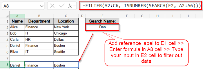
➤ Add reference label to E1 cell such as Search Name:
➤ Pick a blank cell like E2 for your input.
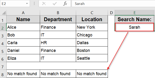
➤ Enter formula in A8 cell to display filtered data: =FILTER(A2:C6, ISNUMBER(SEARCH(E2, A2:A6)))
➤ Type your input in E2 cell such as Dan and press Enter for results to appear.
Create a Search Box Using FILTER Function (Excel 365 & Excel 2021)
If you’re using Excel 365 or Excel 2021, this method is the fastest and most dynamic way to build a real-time search box. It leverages Excel’s modern FILTER function, which updates the displayed data instantly as you type. Perfect for responsive dashboards or live reports, this technique doesn’t require any coding or helper columns.
Steps:
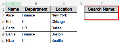
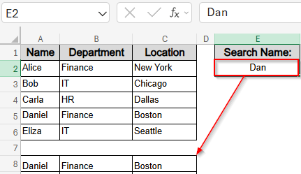
➤ In an empty cell above or next to your data (e.g., E1), type a label like Search Name: and in cell E2, leave it empty for user input.
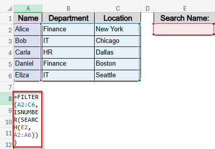
➤ In another cell (e.g., A8), enter this formula:
=FILTER(A2:C6, ISNUMBER(SEARCH(E2, A2:A6)))
➤ Replace A2:C6 with the range of your actual data, and A2:A6 with the column you want to search (e.g., “Name”).
➤ Excel will immediately portray a temporary replica of your filter range.
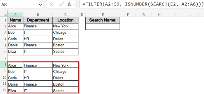
➤ You can search for any name in your data range by typing in E2 cell and it will display the entire matching row starting from A8 cell. For example, we partially typed Dan and hit Enter. Excel scanned all data and has shown us the relevant match.
Use a Drop-Down Search Box with AutoFilter
Looking for a simple way to search your data without writing any formulas? Excel’s AutoFilter tool is your best option. With just a few clicks, you can enable dropdown filters in your headers, and instantly search any column using the inbuilt search bar inside each dropdown. This method is ideal for beginners or quick tasks.
Steps:
➤ Click anywhere inside your dataset. For example, A2 cell.
➤ Go to the Data tab on the ribbon.
➤ Click Filter in the “Sort & Filter” group.
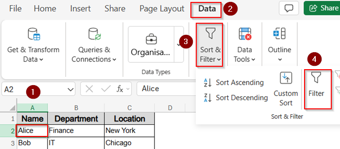
➤ Small dropdown arrows will appear in each header cell.
➤ Click the dropdown arrow on the column you want to search (e.g., Name).
➤ In the search field within the filter box, type your keyword and hit Apply.
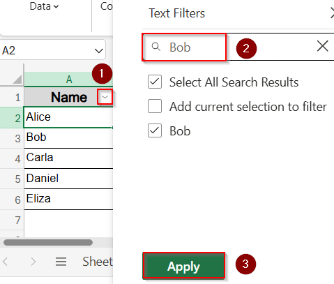
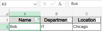
➤ Excel will instantly filter the data to match your typed keyword.
This method is ideal when you want a quick, user-friendly search box without formulas or macros.
Insert a Visual Filter Using Slicers (For Tables or PivotTables)
If you like a more visual and interactive approach, slicers are perfect for you. They allow you to click buttons instead of typing search terms. This is especially useful if you’ve formatted your dataset as an Excel Table or PivotTable. Slicers offer clean, clickable filters ideal for dashboards and reports.
Steps:
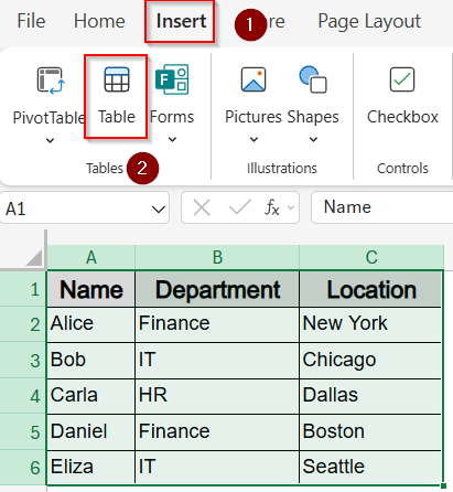
➤ Select your dataset and press Ctrl + T to convert it into a table or go to Insert tab >> Table.
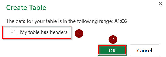
➤ Check My table has headers and click OK.
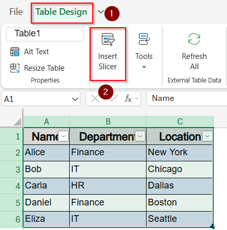
➤ With the table selected, go to the Table Design tab.
➤ Click Insert Slicer.
➤ Choose the column(s) you want to filter (e.g., Name and Department) and click OK.

➤ A slicer box will appear. Click values like Finance and Daniel to filter your dataset instantly.
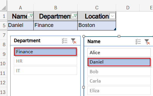
Slicers are intuitive, stylish, and perfect for dashboards or reports.
Build an Interactive Search Box with ActiveX TextBox
If you’re not comfortable with coding but still want an interactive search feature, you can easily create a search box using an ActiveX TextBox and Excel formulas. This method is beginner-friendly and doesn’t require any VBA.
Steps:
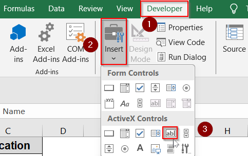
➤ First of all, go to the Developer tab >> Click on Insert >> Choose Textbox under ActiveX controls.
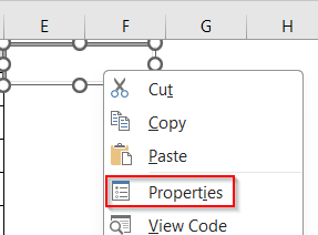
➤ Draw the textbox on your sheet and right-click on it. After that, go to properties
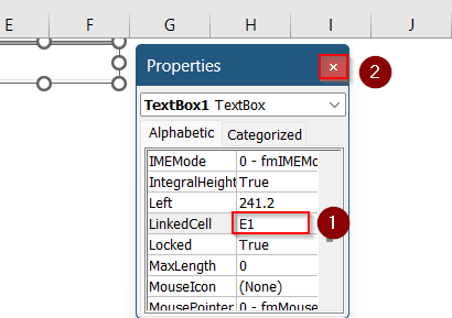
➤ Set Linked cell to E1 and close the pop up.
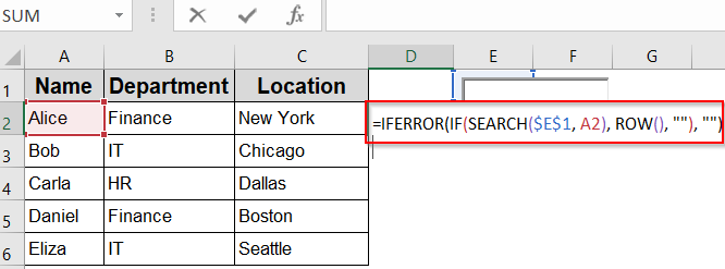
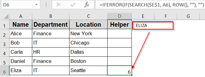
➤ Let column D be your helper column. Enter this formula in D2 cell:
=IFERROR(IF(SEARCH($E$1, A2), ROW(), “”), “”)
This formula checks if the value in cell E1 appears in the Name column (A2:A6). If it does, it returns the row number; otherwise appears blank.
➤ Drag down the formula all the way to D6 using the AutoFill handle.

➤ Now, type your desired value inside the Textbox to run a search. For example, entering Eliza into the Textbox shows the corresponding row number, which is 6.
Perform Multi-Column Search with FILTER + SEARCH + IFERROR
If you want to search across multiple columns (e.g., Name, Department, Location), you can tweak the formula to include more than one condition. This method is great when your search query could appear in any field, not just one specific column.
Steps:
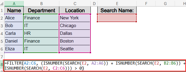
➤ In an empty cell above or next to your data (e.g., E1), type a label like Search Name: and in cell E2, leave it empty for user input.

➤ In another cell (e.g., A8), enter this formula:
=FILTER(A2:C6, (ISNUMBER(SEARCH(E2, A2:A6)) + ISNUMBER(SEARCH(E2, B2:B6)) + ISNUMBER(SEARCH(E2, C2:C6))) > 0)
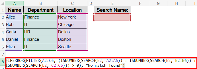
➤ Wrap with IFERROR if needed:
=IFERROR(FILTER(A2:C6, (ISNUMBER(SEARCH(E2, A2:A6)) + ISNUMBER(SEARCH(E2, B2:B6)) + ISNUMBER(SEARCH(E2, C2:C6))) > 0), “No match found”)
➤ Type a name like Bob and information from all columns will become visible to you.
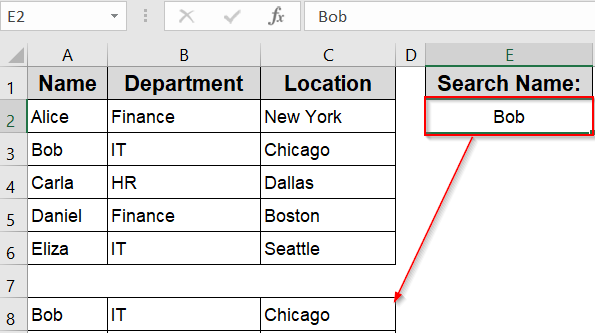
This approach searches across all selected columns simultaneously and returns any matching row and displays No match found if the data doesn’t exist.
Frequently Asked Questions
Can I search more than one column at once?
Yes, you can. To search across multiple columns, you’ll need to adjust the formula to check all those columns using SEARCH or ISNUMBER functions in combination. This allows you to create a more flexible search experience without writing any VBA.
Does this work in older versions of Excel?
Unfortunately, the FILTER function only works in Excel 365 and Excel 2021. If you’re using Excel 2016 or earlier, you’ll need to use AutoFilter, helper columns with formulas like INDEX + MATCH, or consider using a VBA-based approach to replicate the dynamic filtering experience
Can I reset the search box?
Yes, you can reset the search box easily by clearing the linked input cell. If you want a more elegant solution, you can insert a small button linked to a macro that clears the cell automatically.
What’s the easiest method for beginners?
The easiest method for beginners is using AutoFilter with the default dropdowns Excel provides. It requires no formulas, no coding, and works across nearly all Excel versions. Just click the dropdown arrows to filter your dataset by any column value.
Wrapping Up
In this tutorial, we explored multiple ways to create a filtering search box for your Excel data by using formula-based solutions like the FILTER function to interactive ActiveX Controls Textbox. Whether you’re managing a customer list, inventory, or employee records, a search box makes Excel navigation faster and more intuitive. Feel free to download the practice file and share your feedback.