When working with data in different languages, translating multiple cells in Excel manually can be tedious and error-prone. However Excel offers several methods to help you translate text directly within your spreadsheet whether you have a small list or a large dataset, you can efficiently translate multiple cells without needing any online tools or add-ins.
In this article, you’ll learn the best ways to translate multiple cells in Excel using formulas, Power Query, and other built-in tools. These methods work across Excel 2013, 2016, 2019, 2021, and Microsoft Office 365.
Steps to translate multiple cells in Excel:
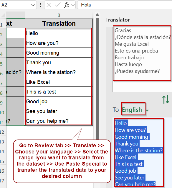
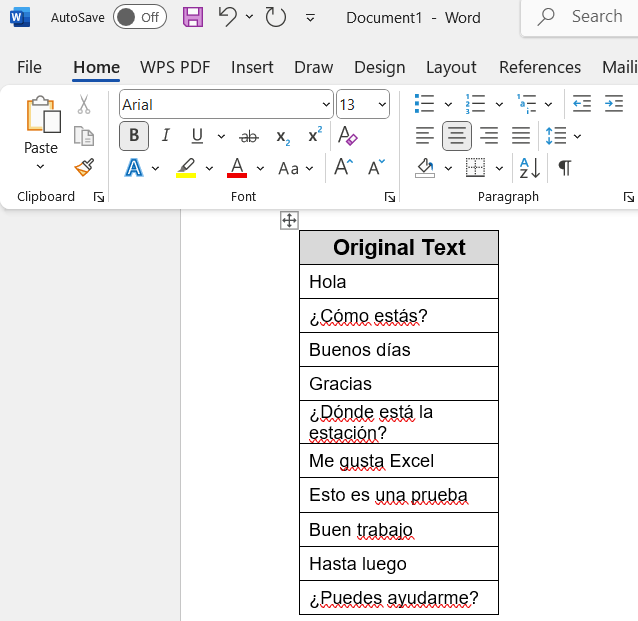
➤ First, select the range of cells you want to translate (e.g., Original Text).
➤ Go to the Review tab in the Excel ribbon, then click Translate in the Language group.
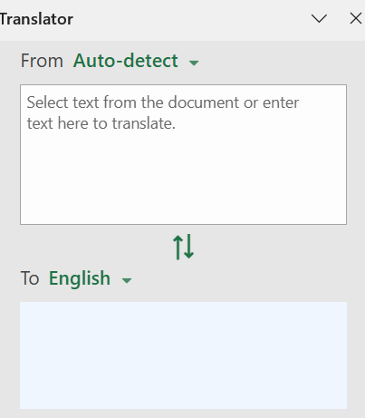
➤ A Research pane or Translator sidebar will appear on the right side of your screen.
➤ In the “To” dropdown, choose the target language you want to translate to (like English, French, etc.)
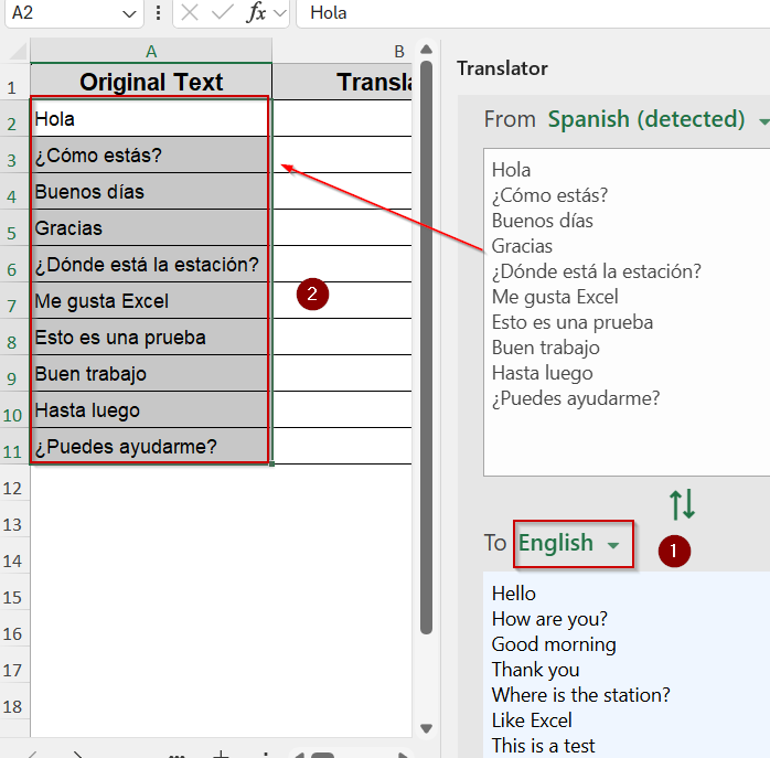
➤ Under “From,” Excel should automatically detect the source language. If not, choose the correct source manually which is Spanish.
➤ Select your desired range which is A2:A7 when you are inside the From box.
➤ Your data will be immediately translated. You can copy the translated data using Ctrl + C .
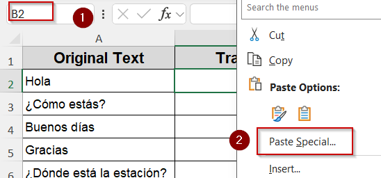
➤ Go back to your sheet and right-click the destination cell such as B2 and select Paste Special.
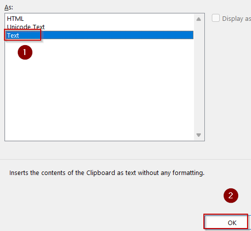
➤ Select Text in the dialog, and hit OK.
Utilize the Built-In Translate Tool in Excel
If you’re using Excel with built-in language tools, you can quickly translate multiple cells directly using the Review tab. This method works well for short phrases and doesn’t require any formulas or add-ins.
Steps:
➤ First, select the range of cells you want to translate (e.g., Original Text).
➤ Go to the Review tab in the Excel ribbon, then click Translate in the Language group.

➤ A Research pane or Translator sidebar will appear on the right side of your screen.
➤ In the “To” dropdown, choose the target language you want to translate to (like English, French, etc.)
➤ Under “From,” Excel should automatically detect the source language. If not, choose the correct source manually which is Spanish.
➤ Select your desired range which is A2:A7 when you are inside the From box.
➤ Your data will be immediately translated. You can copy the translated data using Ctrl + C .
➤ Go back to your sheet and right-click the destination cell such as B2 and select Paste Special.
➤ Select Text in the dialog, and hit OK.
Now your translation column is filled sequentially in your worksheet.
![]()
Note:
This method is best for small lists and short phrases. It doesn’t translate all selected cells at once, so you must review and copy them individually.
Convert Large Tables via Microsoft Word’s Translator (Offline Option)
If Excel’s built-in translation functions fall short, especially for full tables, then Microsoft Word offers a reliable workaround to translate entire Excel datasets quickly.
Steps:
➤ Copy your table from Excel using Ctrl + C and paste into Word using Ctrl + V .
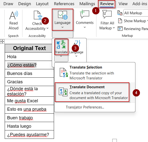
➤ Go to the Review tab >> Click on Translate under the Language group in Word.
➤ Select Translate Document from the list of options.
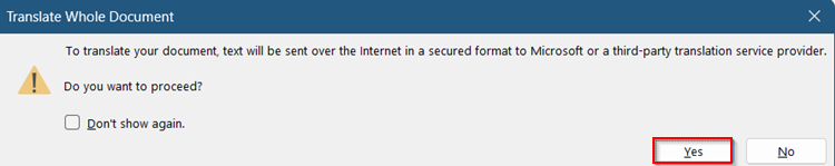
➤ Click Yes in the confirmation pop-up to proceed.
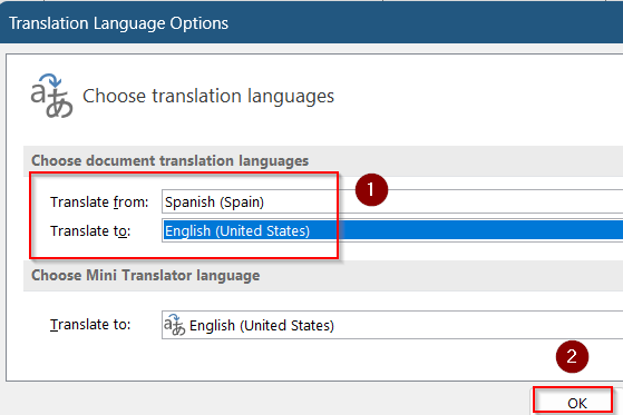
➤ Choose your Translate From and To languages and click OK in the dialog.
➤ Once the translation is complete, copy the table from Word using Ctrl + C .
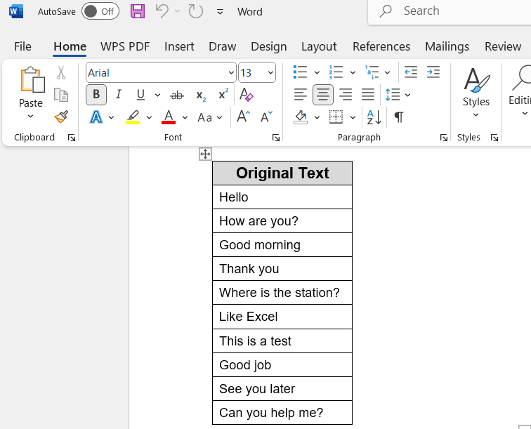
➤ Then, paste it back into Excel using Ctrl + V in the Translation column.
This method is great for translating large blocks of structured data all at once when Excel can’t handle it natively.
Apply TRANSLATE and DETECTLANGUAGE Functions (Microsoft 365 Only)
Excel’s built-in TRANSLATE and DETECTLANGUAGE functions let you identify the language of your text and translate it directly inside your worksheet. You can use these functions to build dynamic multilingual spreadsheets quickly.
Steps:
➤ In a blank cell, start typing the formula:
=TRANSLATE(
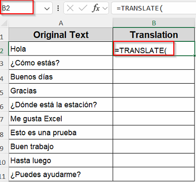
and select the cell containing the text (e.g., A2).
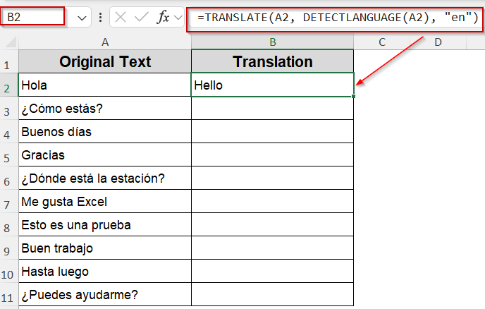
➤ To detect the source language automatically, leave the second argument blank, or explicitly use DETECTLANGUAGE function in a corresponding cell like B2 to detect and translate dynamically:
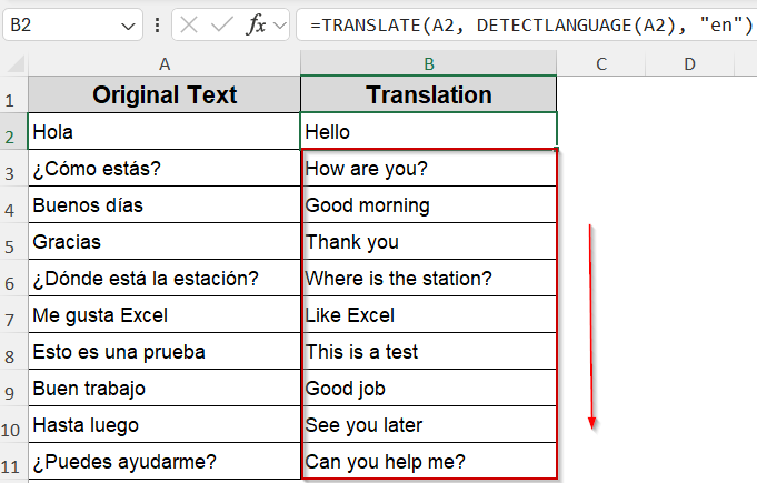
=TRANSLATE(A2, DETECTLANGUAGE(A2), “en”)
➤ Use the AutoFill handle to drag it below B2 cell.
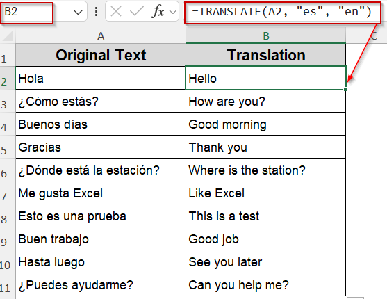
➤ Alternatively, if you know the source language, enter the language code (e.g., “en” for English) as the second argument:
=TRANSLATE(A2, “es”, “en”)
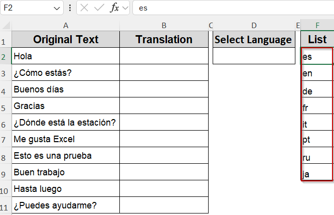
➤ To make the target language dynamic, create a dropdown with supported language codes like en, de, es, fr, it, pt, ru, ja in column F. Then, name the column List.
➤ Select a blank cell where your drop-down should appear (e.g., D2). Go to the Data tab >> Data Validation under Data Tools.
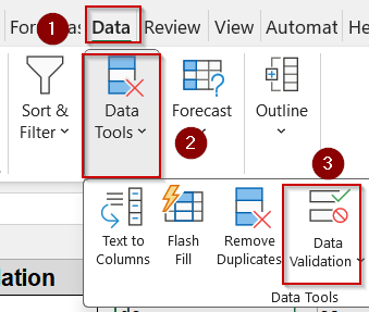
➤ Set Allow to List and type in Source box:
=$F2:$F9
➤ Click OK.
![]()
➤ Select your language code such as en for English in D2 cell from the drop-down we created.
![]()
➤ Use this formula in B2 cell:
=TRANSLATE(A2, DETECTLANGUAGE(A2), $D$2)
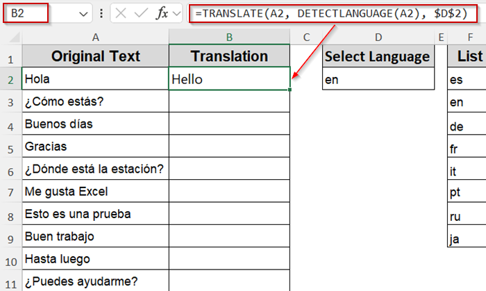
Here, $D$2 is used to lock the reference so you can drag the formula down using the AutoFill handle.
![]()
➤ To simply detect the language without translation, use formula:
=DETECTLANGUAGE(A2)
![]()
Excel returns the short language code, such as “en” for English or “es” for Spanish.
Use Power Query to Convert Text with Google API
This method uses Power Query and a custom formula to connect with Google Translate and fetch live translations. It’s ideal if you’re translating multiple rows and are connected to the internet.
Steps:
➤ Select both columns (Original Text and Translation).
➤ Go to the Data tab and click From Table/Range under the Get & Transform group.
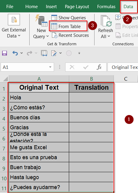
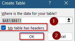
➤ Check “My table has headers” and press OK to launch Power Query Editor.
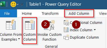
➤ Click the Add Column tab, then choose Custom Column.
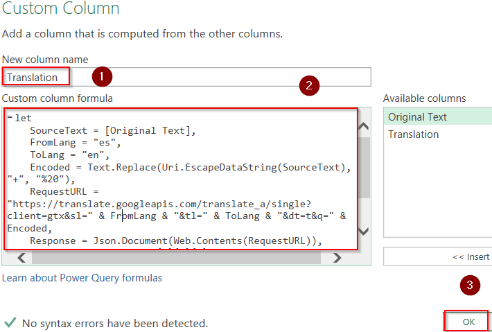
➤ Name the new column as Translation.
➤ Paste this full formula into the formula box:
let
    SourceText = [Original Text],
    FromLang = "es",
    ToLang = "en",
    Encoded = Text.Replace(Uri.EscapeDataString(SourceText), "+", "%20"),
    RequestURL = "https://translate.googleapis.com/translate_a/single?client=gtx&sl=" & FromLang & "&tl=" & ToLang & "&dt=t&q=" & Encoded,
    Response = Json.Document(Web.Contents(RequestURL)),
    Translation = Response{0}{0}{0}
in
    Translation
➤ To customize this code, change the FromLang and ToLang values (e.g., “fr” for French, “de” for German). Also update [Original Text] if your column has a different name.
➤ Press OK to apply.
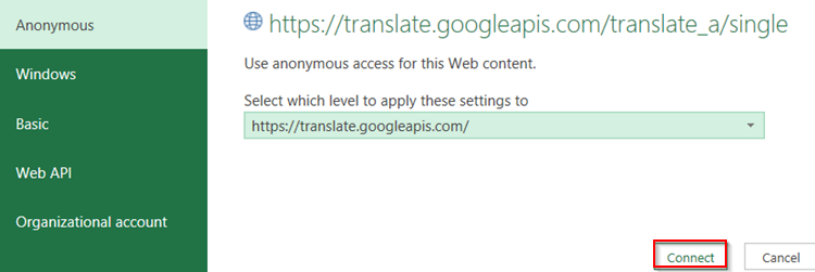
➤ Click the Connect button on the dialog to approve internet connection.
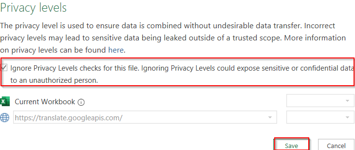
➤ Check the box to Ignore Privacy Level checks and hit Save.
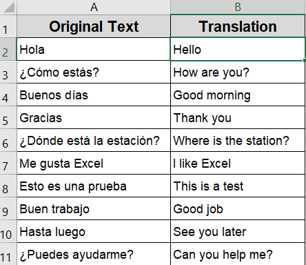
➤ The new column will automatically fill with translations from Google.
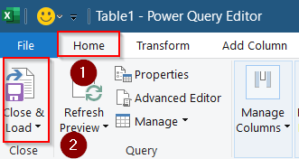
➤ Go to Home tab >> Click Close & Load to return the results to your Excel sheet.
➤ Then, your translation column is exported to a new sheet.
![]()
➤ To automatically refresh the table, head to the Data tab >> Go to Properties under Queries & Connections group >> Click the small button beside Name in the first dialog and check Refresh data when opening the file and hit OK.
![]()
Now you have a dynamic translation table in your worksheet connected directly with Google Translate.
Frequently Asked Questions
Does Excel have a built-in function for translating multiple cells at once?
No, Excel only provides single-cell translation using the TRANSLATE function. For multiple cells, use formulas, Power Query, or third-party tools to batch the process.
Can I translate Excel data without an internet connection?
Yes, you can copy data to Microsoft Word and use its offline translator. Excel’s online functions like TRANSLATE and Power Query API require an internet connection.
What if the DETECTLANGUAGE function returns the wrong code?
DETECTLANGUAGE function uses automatic detection. If it returns the wrong result, you can manually input the source language code in the TRANSLATE formula to override the detection.
Why is my translation column returning errors?
Check for empty cells, invalid language codes, or special characters. Ensure the formula uses text inputs and references valid cells with actual phrases to avoid errors.
Can I change the language after applying the translation?
Yes. If you’re using a dropdown with language codes, changing the dropdown value will automatically update the translated results using dynamic formulas across your dataset.
Wrapping Up
In this tutorial, we covered several effective methods to convert multiple cells in Excel using the Translate tool, Microsoft Word, built-in functions, and Power Query with the Google Translate API. Whether you’re translating a few cells, creating a dynamic multilingual table, or automating the process for a larger dataset, each method is suited to a different need. Feel free to download the practice file and share your feedback.