How to Format Numbers as Millions in Google Sheets

Working with large numbers in spreadsheets can get messy, especially when you’re dealing with thousands or millions in financial reports, marketing data, or performance dashboards. Instead of clogging up cells with long digits like 6,000,000, it’s much cleaner to display them as 6M. Google Sheets lets you do this using custom number formatting & formulas.

In this article, you’ll learn how to format numbers into millions in Google Sheets using different methods. Each approach has its benefits depending on how dynamic or automated you want your data display to be.

What Does Formatting Numbers as Millions Mean?

Formatting numbers into millions is a technique that helps simplify how data is displayed. Instead of showing full-length numbers like 1,200,000, you can display them as 1.2M. It’s particularly helpful when working with financial figures, budgeting sheets, sales numbers, or any dataset that involves large values. This makes the spreadsheet look cleaner and helps readers focus on the actual value instead of counting zeros.

If you’re working with large numbers in your spreadsheet, displaying them as “M” (for millions) can make your data much easier to scan, especially in reports, dashboards, or presentations. Instead of showing full values like 6,000,000, this method lets you format numbers to appear as 6M right in the same cell, while keeping the original value intact for calculations.

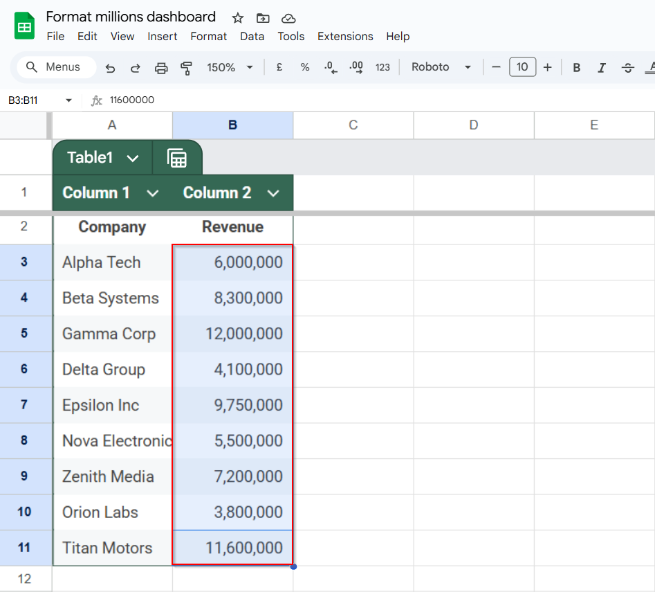
In the example below, we’re working with a dataset that lists different companies and their revenue.

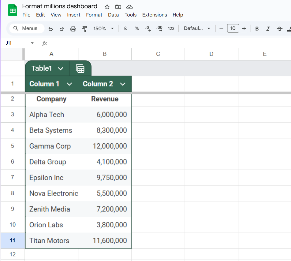
We’ll apply a custom number format to the Revenue column so values like 6,000,000 appear as 6M in a cleaner format.

Steps:

➤ Select the cells you want to format (e.g., B3:B11).

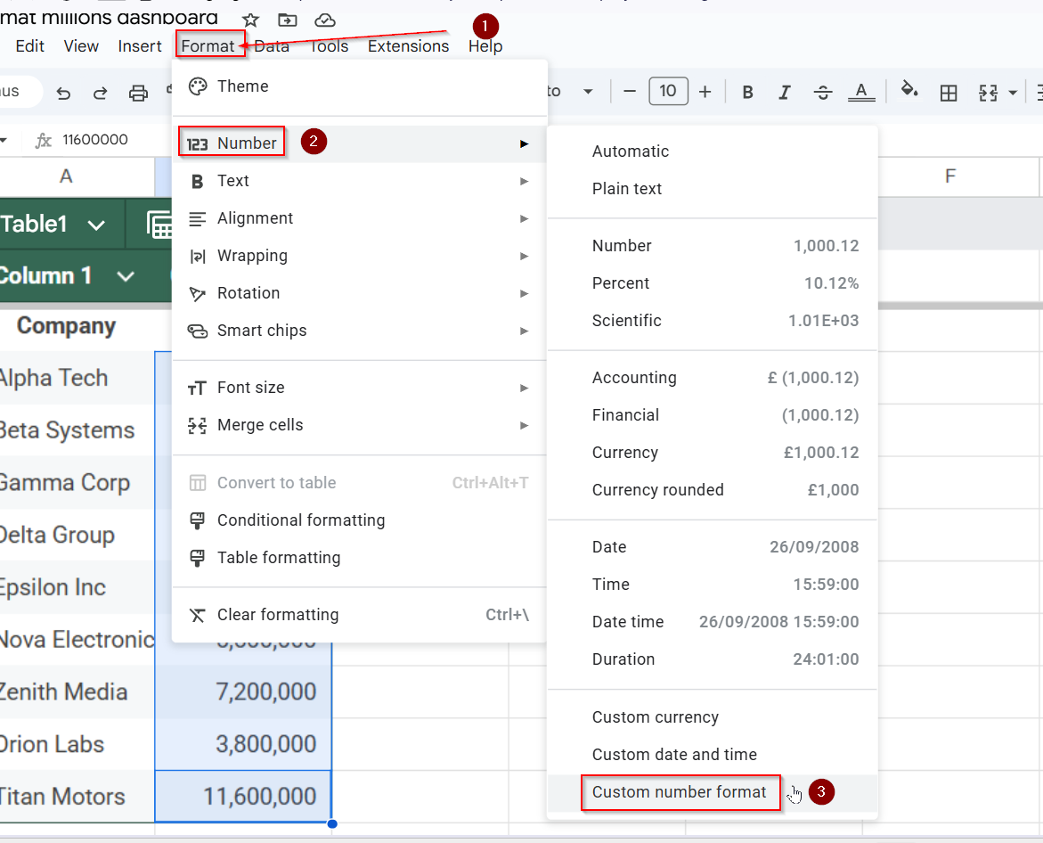
➤ Click Format >> Number >> Custom number format.

➤ Enter this format code: #,##0,,”M”

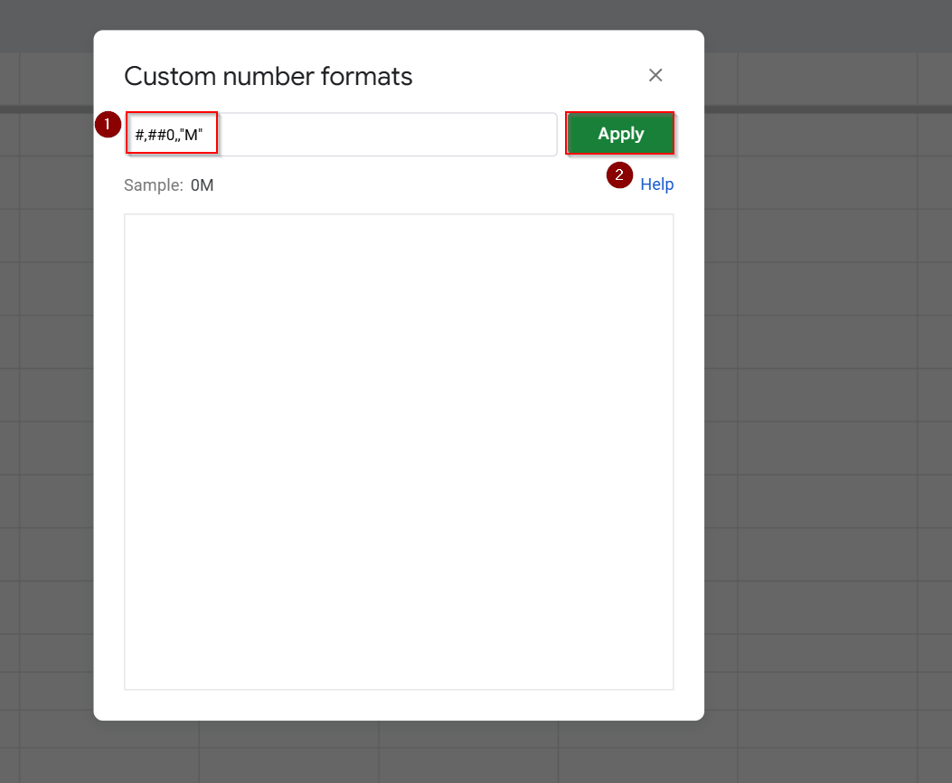
➤ Click Apply.

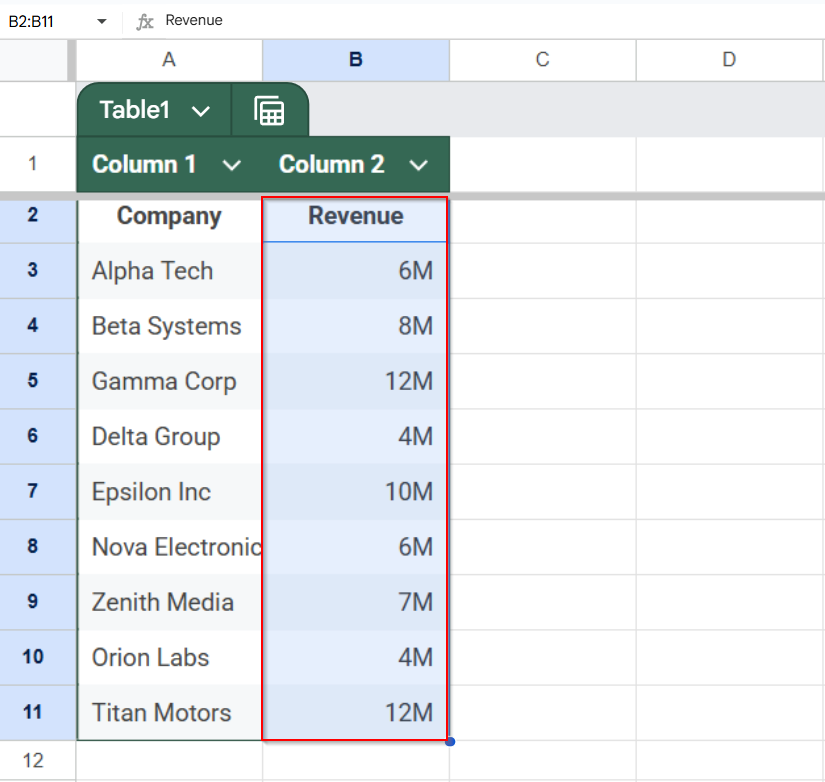
The double commas (,,) tell Google Sheets to divide the number by 1,000,000. The “M” at the end displays the unit.

In this method, we’ll create an extra column that displays your numbers in millions by dividing the original values by one million. This is perfect if you want to keep the full numbers intact for calculations, but also want a cleaner, easier-to-read version for viewing or sharing.

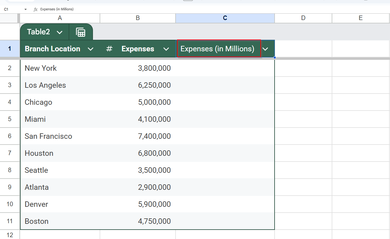
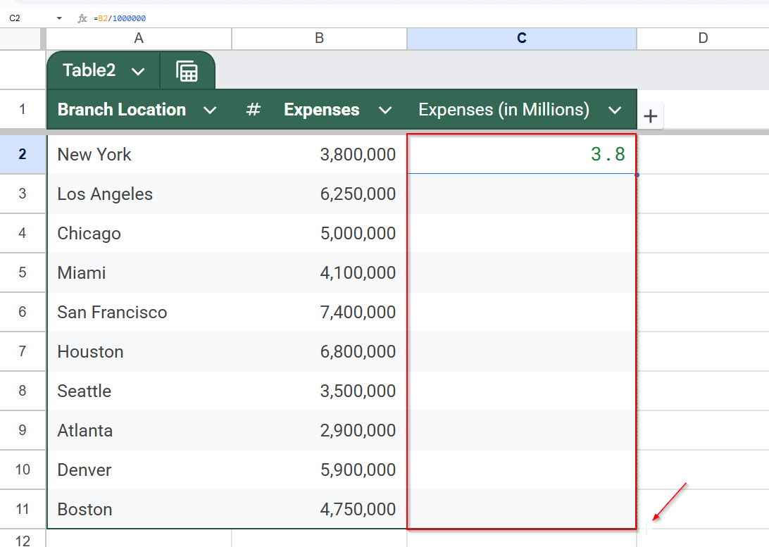
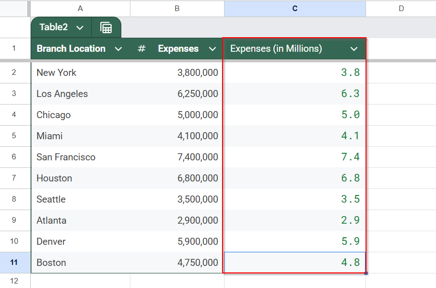
For this example, we’re working with a dataset that shows monthly expenses for different branch locations across the U.S. Each value is in full form (like 3,800,000), and we’ll use a helper column to convert them into a simplified format like 3.8. This makes the sheet easier to understand, especially helpful for dashboards, presentations, or when summarizing financial reports.

Steps:

➤ Insert a new column (e.g., Expenses in Millions).

➤ In the first cell of the new column (e.g., C2), enter:

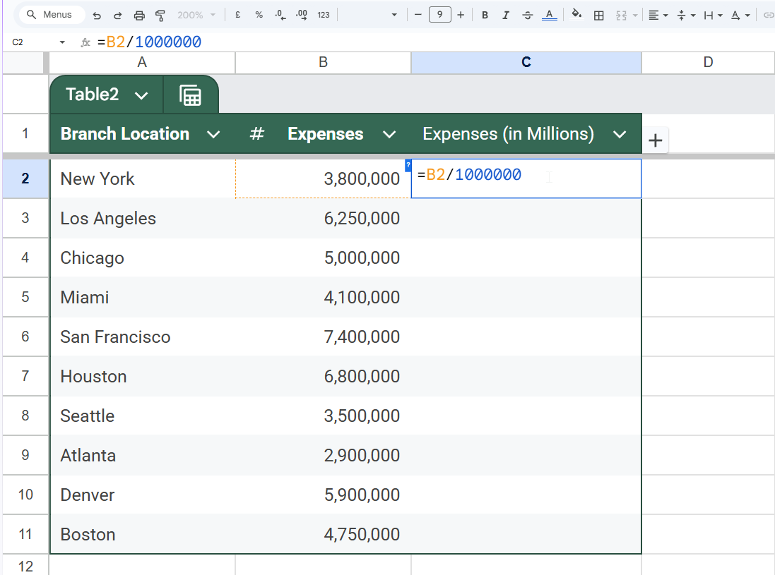
➤ Drag down to apply it to the rest of the cells.

➤ Format the new column to show one decimal: Format >> Number >> Custom number format

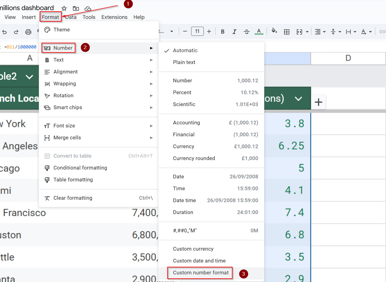
➤Enter 0.0 in the box to make it neater (e.g., 3.8 instead of 3.800000).

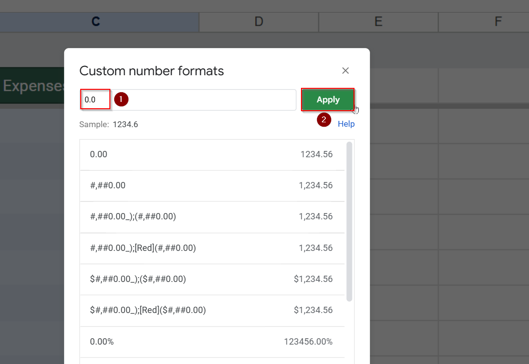
➤ Click on Apply.

This method keeps your original data intact while showing a cleaner, easier-to-read version in millions.

If you want more control over how the numbers appear in each cell (for example, showing “7.3M” instead of 7,300,000), you can use the TEXT function. This method lets you customize the display format without changing the original data.

It’s beneficial for creating clear and concise reports or presentations where simplified figures make the information easier to understand.

Steps:

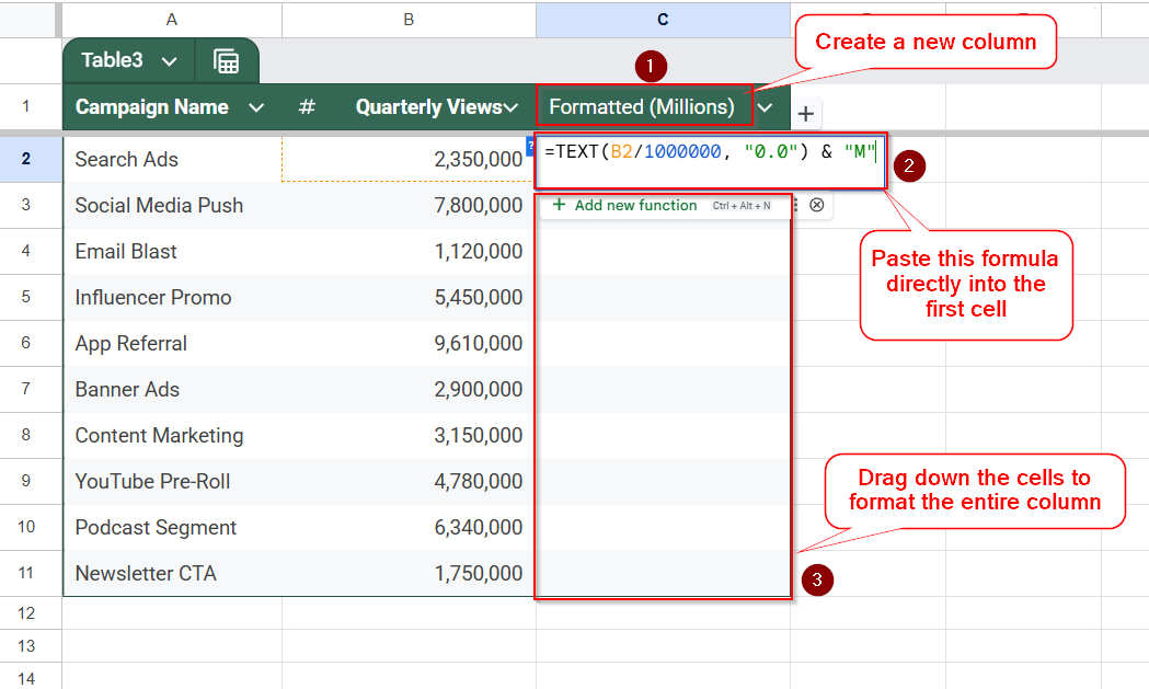
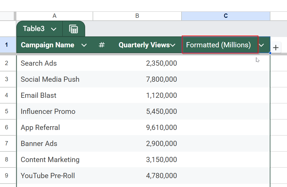
➤ Insert a new column next to Quarterly views.

➤ In C2 cell, enter:

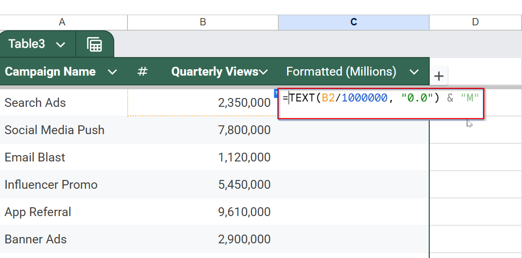
➤ Drag to apply across rows.

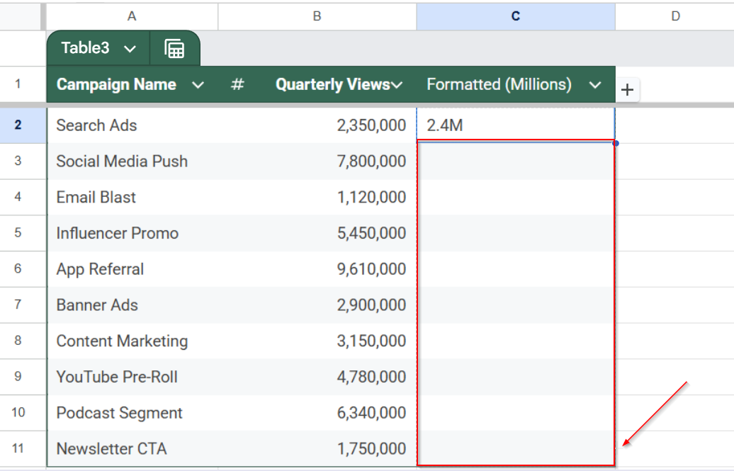
Now you have a visual “millions” version alongside the raw number.

Frequently asked questions

Will formatting numbers as millions affect my calculations?

No, formatting numbers as millions only changes how the numbers look, not their actual values. Your calculations and formulas will still use the full original numbers, so results remain accurate while the display becomes easier to read.

Is there a way to automatically update the display if the numbers change?

Yes, the display updates automatically when the original numbers change if you use formulas like dividing by 1,000,000 or the TEXT function. This ensures your formatted numbers always reflect the latest data without needing manual adjustments.

Is it possible to apply million formatting to a large range of cells at once?

Yes, you can apply formatting to multiple cells by selecting the desired range before setting the custom number format or formula. This bulk application saves time and ensures consistency across your spreadsheet. However, if you have data across different sheets, you will need to apply formatting individually or use formulas referencing named ranges.

Can I format numbers as thousands (e.g., 6K) instead of millions?

Yes, Google Sheets allows you to customize formats quickly. To display numbers in thousands, you can use a custom format like  #,##0,”K”, or adjust your formulas to divide by 1,000 instead of 1,000,000. This flexibility helps you adapt your spreadsheet to different data scales without re-entering values.

Wrapping up

Formatting numbers into millions in Google Sheets can make your spreadsheets cleaner and easier to read, especially when you’re dealing with big numbers in reports. Whether you choose to use custom formats, formulas, or helper columns, each method gives you flexibility based on your use case. Give them a try and see which one works best for your data.