Identifying all cells that contain a specific value is a common task when working with large datasets in Google Sheets. Whether you’re tracking down duplicate entries, searching for key terms, or filtering out relevant data, Google Sheets offers several functions and tools to help you locate matching values with precision and flexibility.
This article walks you through the most effective methods to find all cells with a specific value in Google Sheets. From formula-based approaches like LOOKUP, VLOOKUP, INDEX + MATCH, to visual techniques like conditional formatting and interactive filters, you’ll learn multiple ways to uncover, highlight, and analyze data that matches your criteria.
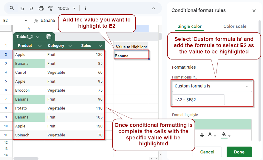
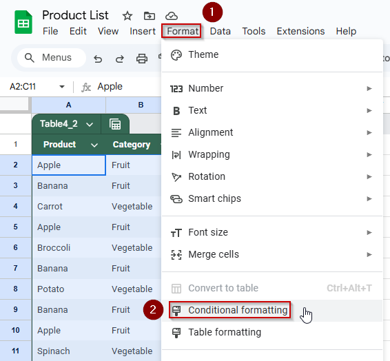
Steps to highlight all cells with a specific value using Conditional Formatting in Google Sheets:
➤ Select the data range (e.g., A2:C11) you want to search within.
➤ Go to Format >> Conditional formatting.
➤ Choose Custom formula is and enter the formula =A2 = $E$2 (where E2 contains your lookup value).
➤ Pick a highlight color and click Done.
➤ All matching cells will be instantly highlighted, making it easy to spot specific values visually.
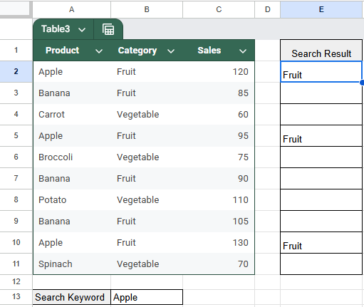
Extract Matching Values Using ARRAYFORMULA Function
The ARRAYFORMULA function in Google Sheets enables you to apply a formula to an entire range of cells at once, making it a powerful tool for finding all cells that match a specific value. By combining ARRAYFORMULA with a logical test like IF, you can quickly scan a column, compare each cell against a target value, and return only the matching entries. This method is dynamic and efficient, allowing you to create a filtered view of your data without altering the original dataset.
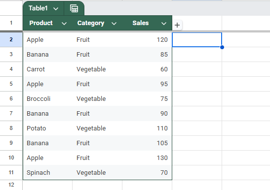
Here is the sample dataset we will be using for this article:
Steps:
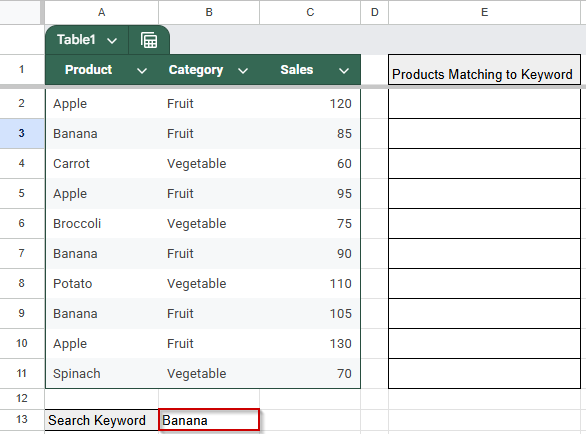
➤ In cell B13, enter the value you want to search for, for example: Banana
➤ In cell E2 (Or, anywhere you like), enter the following formula to find matching products in column A:
=ARRAYFORMULA(IF(A2:A11 = B13, A2:A11, “”))
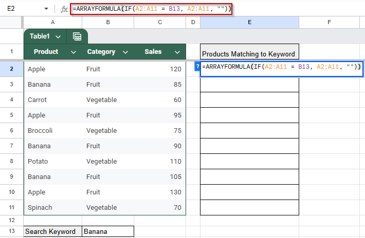
➤ Press Enter.
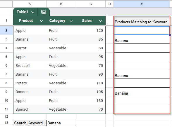
This method is ideal for quickly identifying all instances of a value in a list and works well when integrated into dynamic spreadsheets or dashboards.
Retrieve Data Related to Specific Value Using VLOOKUP Across a Range
VLOOKUP is one of the most commonly used functions in Google Sheets for finding associated values based on a match in the first column of a range. However, it’s important to note that VLOOKUP is designed to return the first matching result only. To simulate finding all cells with a specific value using VLOOKUP, you can apply it across multiple rows using ARRAYFORMULA. This lets you retrieve corresponding data, like sales figures, for each instance of a matching value.
Steps:
We will use the same dataset from the first method.
➤ In cell B13, enter the value you want to search for, such as: Banana

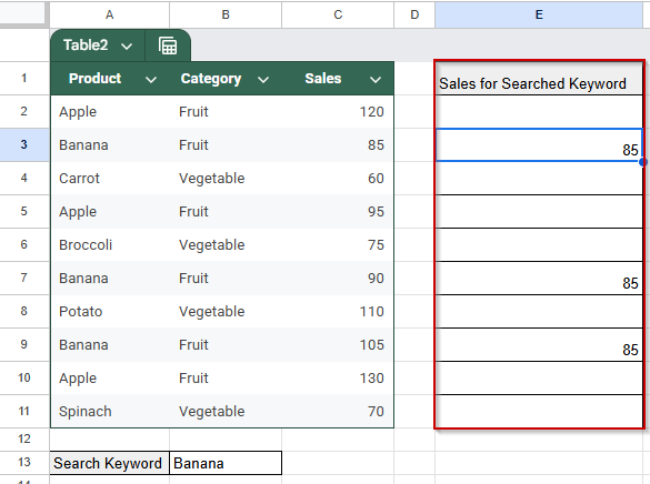
➤ In column F, we will retrieve the sales values related to each occurrence of “Banana”. In cell F2, enter:
=ARRAYFORMULA(IF(A2:A11 = E1, VLOOKUP(A2:A11, A2:C11, 3, FALSE), “”))
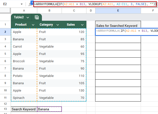
➤ Press Enter.
Find Related Cells to Specific Value with the INDEX-MATCH Function Combination
The INDEX and MATCH functions together provide a flexible way to look up values in Google Sheets. Unlike VLOOKUP, which requires the lookup value to be in the first column, INDEX-MATCH can search any column and return data from any other column in the dataset. While this combination normally returns a single result, it can be adapted with ARRAYFORMULA and logical tests to find all cells matching a specific value and retrieve related data.
Steps:
➤ In cell B13, enter the value to search for, such as: Apple
➤ To retrieve the Category for all rows where the product equals the search value, enter this formula in cell E2:
=ARRAYFORMULA(IF(A2:A11 = B13, INDEX(B2:B11, ROW(A2:A11) – ROW(A2) + 1), “”))
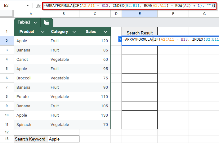
➤ Press Enter.
This method is useful when you want to flexibly retrieve related information from any column based on matching criteria in another column.
Count All Non-Empty Cells With Values Using COUNTA Function
If your goal is to quickly find out how many cells in a column contain any value, not just a specific one, the COUNTA function is the simplest and most efficient solution. COUNTA counts all non-empty cells within a given range, regardless of the data type, including numbers, text, and formulas with results.
This method is ideal when you want a summary metric showing how many entries are present in a column, such as how many products were listed, how many sales records are recorded, or how many categories have been filled in.
Steps:
➤ In cell E1, enter the label: Total Products
➤ In cell E2, enter the formula:
=COUNTA(A2:A11)
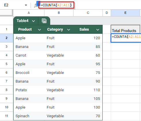
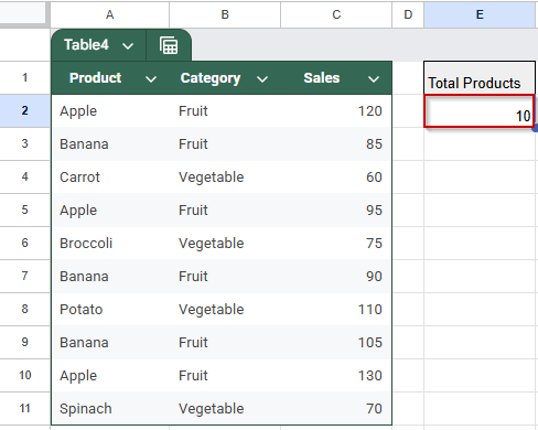
This formula counts all non-empty cells in the range A2:A11, which corresponds to the Product column.
➤ Press Enter.
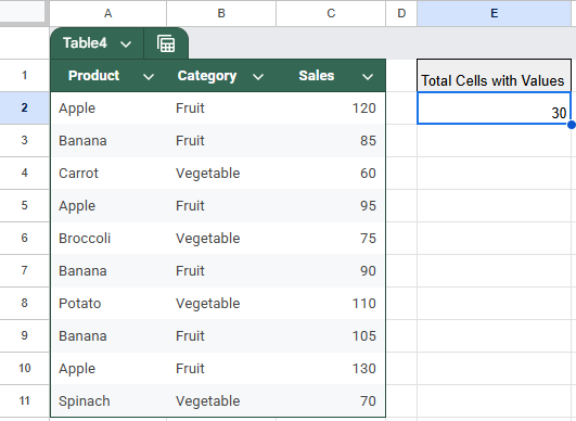
You can use the same approach to count non-empty cells in the whole table. For example, use =COUNTA(A2:C11) to count all filled entries. This is a helpful method when cleaning data or validating whether a dataset is complete.
List All Cell Values in a Single Column Using FILTER and FLATTEN
When you’re working with data across several columns and want to create a single, consolidated list of all the filled values, the combination of the FILTER and FLATTEN functions in Google Sheets is a practical and flexible solution. FLATTEN takes a multi-column range and turns it into a single column, while FILTER can be added to exclude blank cells from the result.
This method is great for creating dropdown menus, validation lists, or searchable references from a table without manually copying and cleaning the data.
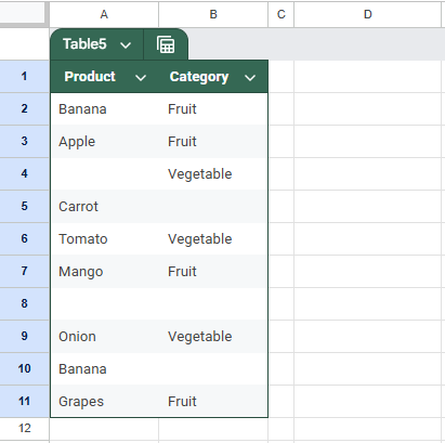
This is an updated dataset we are using for this method.
Steps:
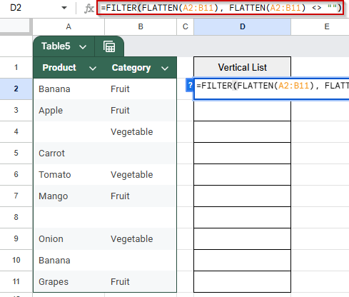
➤ In cell D2, enter the formula:
=FILTER(FLATTEN(A2:B11), FLATTEN(A2:B11) <> “”)
➤ Press Enter.
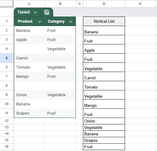
The list updates automatically if values in A2:B11 change.
Highlight Matching Cells with Conditional Formatting
If you want to visually identify all cells that contain a specific value across your dataset, conditional formatting is the most effective tool. Instead of returning results in a new column, this method highlights all matching cells directly in the original range, making it ideal for quick scanning and visual analysis. The formatting updates dynamically as you change the lookup value, helping you explore your data interactively without altering any formulas or structure.
Steps:
➤ Enter the value you want to highlight in E2.
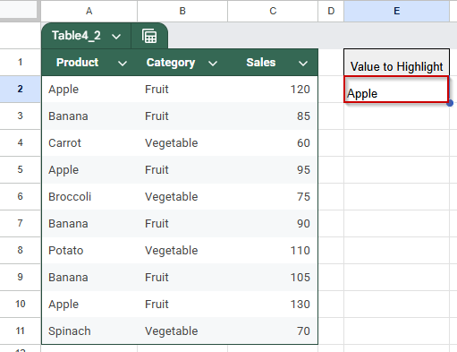
➤ Select the range you want to check, for example, A2:C11.
➤ Go to Format >> Conditional formatting.
➤ Under the “Format cells if” dropdown, choose Custom formula is.
➤ Enter the formula:
=A2 = $E$2
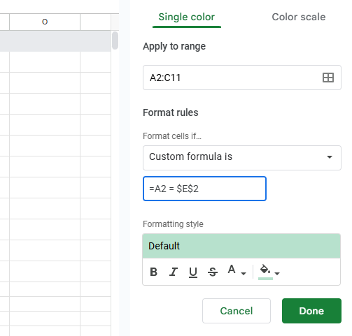
This assumes E2 contains the value you want to highlight (e.g., Apple).
➤ Choose a highlight color under “Formatting style”.
➤ Click Done.
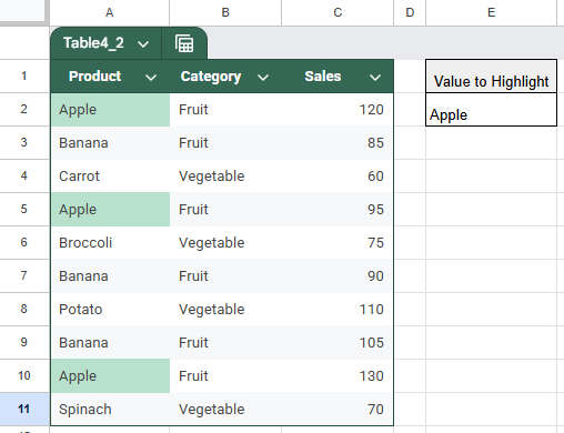
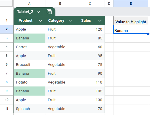
➤ All cells in the selected range that match the value in E2 will now be highlighted automatically.
Frequently Asked Questions
How do I find all cells with a specific value in Google Sheets?
You can use formulas like ARRAYFORMULA, FILTER, VLOOKUP, or a combination of INDEX and MATCH to find and display all cells matching a value. If you prefer a visual method, conditional formatting can highlight them directly in the sheet.
Can LOOKUP return multiple matching results?
No, the standard LOOKUP function only returns a single value—usually the last match found. To return multiple results, you should use ARRAYFORMULA with IF, or the FILTER function.
What’s the difference between COUNTA and COUNT?
COUNTA counts all non-empty cells (including text, numbers, and formulas), while COUNT only includes numeric values. Use COUNTA when you want to count any kind of filled data.
Is FLATTEN available in all Google Sheets accounts?
Yes, FLATTEN is a native function in Google Sheets and doesn’t require any add-ons or extensions. It works best when paired with FILTER to clean up the output.
Wrapping Up
Google Sheets offers several effective ways to find all cells with a specific value, whether you want to extract, count, highlight, or list them. Using formulas like ARRAYFORMULA, FILTER, or conditional formatting, you can build flexible, dynamic tools for analysis. Each method serves a different purpose, so choose the one that best fits your workflow and data needs for faster, clearer decision-making and more accurate, insight-driven spreadsheet results.