In Google Sheets, there are times when you want a formula to reference different cells based on user input or logic, without manually updating the formula. This is where dynamic cell referencing becomes incredibly powerful.
In this article, we’ll explore how to create flexible, changeable cell references using functions like INDIRECT, ADDRESS, and user-driven inputs. This allows you to pull data from various locations based on values in other cells.
Steps to fetch department names from another workbook based on Employee ID:
➤ In the destination workbook, click on your desired cell.
➤ Enter the formula:
=VLOOKUP(A2, IMPORTRANGE(“https://docs.google.com/spreadsheets/d/WORKBOOK1_ID/edit”, “Sheet1!A:C”), 3, FALSE)
➤ Replace WORKBOOK1_ID with the actual Sheet ID from the source Workbook URL. Also change the cell reference from where you will be pulling the data from.
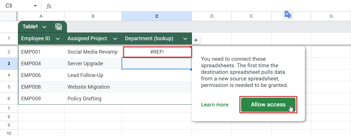
➤ Press Enter. You’ll see a #REF! error initially.
➤ Click the Allow access button to authorize the data connection between the two sheets.
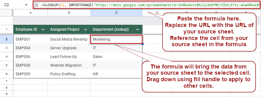
➤ The department for the given Employee ID will appear in cell C2.
➤ Use the fill handle to drag the formula down to apply it to the rest of the rows (e.g., C3 to C11).
➤ The department field will now update automatically whenever Workbook 1 is updated.
Fetch Department Dynamically Using IMPORTRANGE and VLOOKUP Functions in Google Sheets
One of the most powerful ways to reference data across workbooks in Google Sheets is by combining the IMPORTRANGE function with VLOOKUP. This method allows you to dynamically pull a department name from another spreadsheet based on a matching Employee ID. This is perfect for cases where you manage staff in one sheet and project assignments in another.
You’re managing two different spreadsheets:
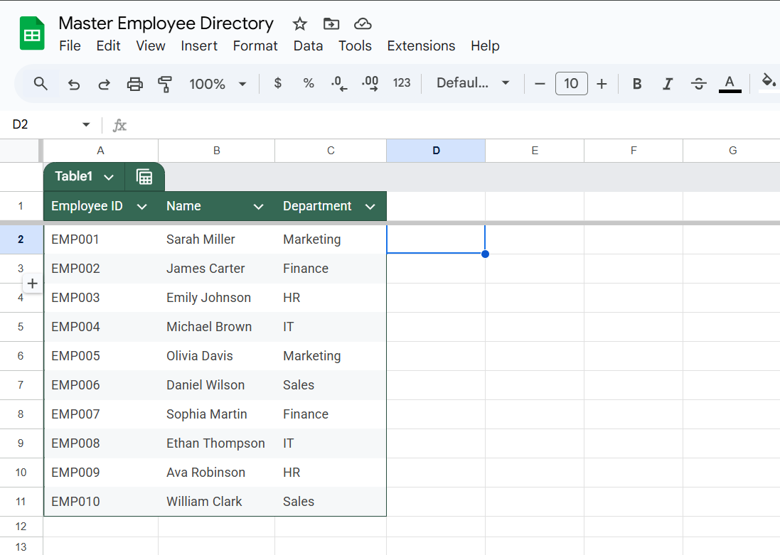
- Workbook 1 (Employee Directory) contains each employee’s ID, name, and department.
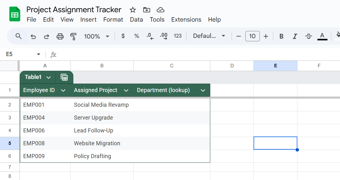
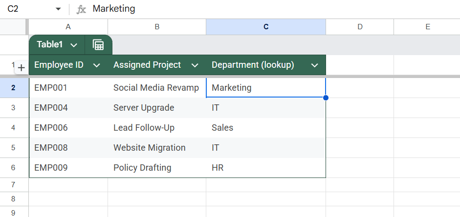
- Workbook 2 (Project Assignment Tracker) lists employee IDs and assigned projects, and you want to pull in their corresponding departments from Workbook 1 automatically.
Let’s now walk through how to fetch the Department values dynamically in Column C of Workbook 2.
Steps:
➤ Open Workbook 2 (Project Assignment Tracker) where you want to fetch the department names.
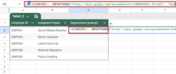
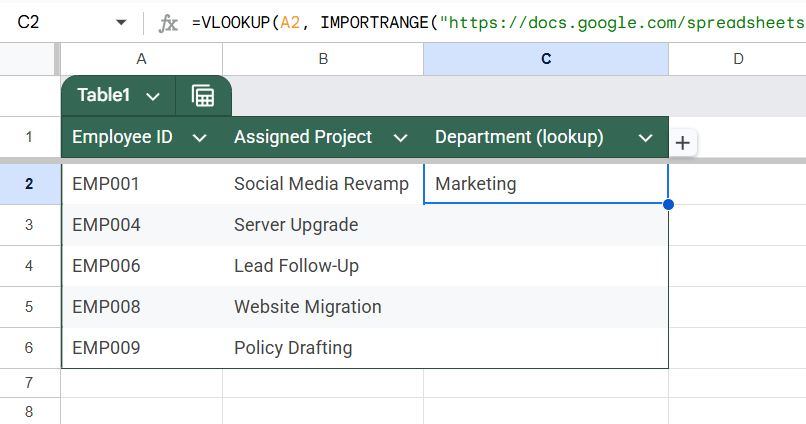
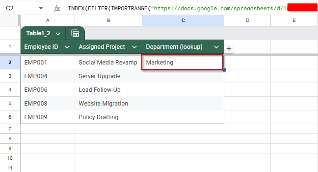
➤ Click on cell C2, where the first department name will appear.
➤ Enter the following formula:
=VLOOKUP(A2, IMPORTRANGE(“https://docs.google.com/spreadsheets/d/WORKBOOK1_ID/edit”, “Sheet1!A:C”), 3, FALSE)
Replace WORKBOOK1_ID with the actual ID from the URL of your Employee Directory. For example, if your link is: https://docs.google.com/spreadsheets/d/1aBcD123EXAMPLEid456/edit#gid=0
Then use 1aBcD123EXAMPLEid456 as a reference to the ID in the formula.
➤ After entering the formula, you’ll likely see a #REF! error. Hover over the cell, and you’ll see an “Allow access” button.
➤ Click Allow access to authorize the connection between the two workbooks.
➤ Once authorized, the department corresponding to the Employee ID in A2 will appear in C2.
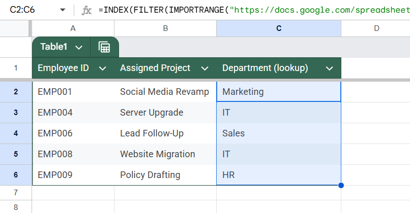
➤ Now, drag the fill handle down from C2 to C11 to apply the same formula to the rest of the rows.
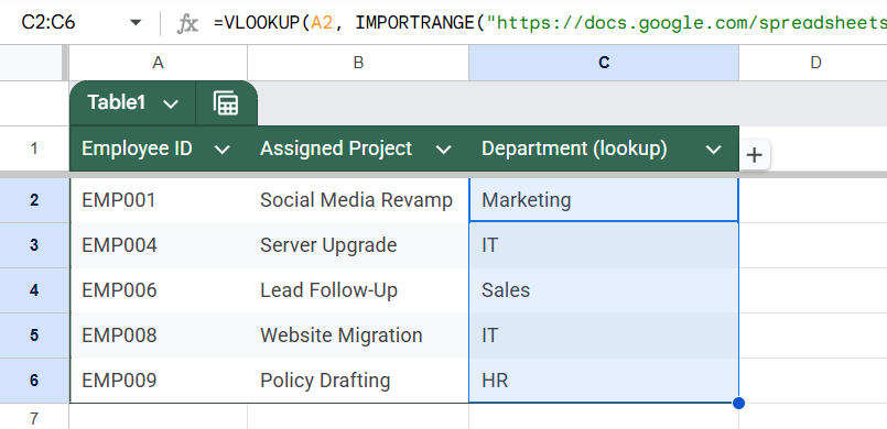
Each row will now display the department fetched from Workbook 1 based on the Employee ID in Column A. This method is dynamic, so any changes made in Workbook 1 (like department updates) will be reflected automatically in Workbook 2.
Use IMPORTRANGE and FILTER Functions to Dynamically Match Employee Data
Another effective and readable way to fetch data from another Google Sheets workbook is by using the FILTER function combined with the IMPORTRANGE function. This method is excellent when you want to return data based on a condition, in this case, the Employee ID. It’s beneficial when you prefer function clarity over nested lookup logic or want to expand to multiple matches.
Steps:
➤ Open Workbook 2 (Project Assignment Tracker)
➤ Click on cell C2, where the department for the first employee will be displayed
➤ Paste the following formula:
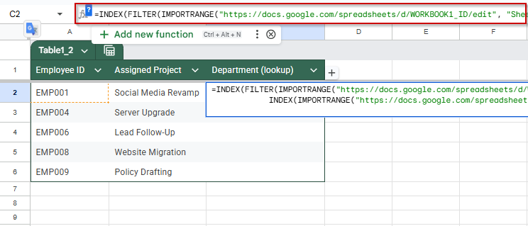
Replace WORKBOOK1_ID with the actual ID from your Employee Directory spreadsheet
➤ FILTER(..., A:A = A2) filters only the row where Employee ID matches the one in Column A
➤ INDEX(..., 1, 3) extracts the Department column from that row.
➤ When the formula is first entered, a #REF! error will appear with a prompt to Allow access

➤ Once permission is granted, the correct department will show up in cell C2
➤ Use the fill handle to drag the formula down from C2 to C11 to fetch department info for all employees
Automatically Fetch Data from Another Workbook by Employee ID Using Apps Script
If you prefer automation or want to fetch data programmatically, Google Apps Script offers a powerful way to connect two Google Sheets. In this method, we’ll write a script in Workbook 2 (Project Assignment Tracker) that pulls the department name for each employee based on their ID from Workbook 1 (Employee Directory).
This is helpful for larger datasets or when you want the process triggered by a button or menu item.
Steps:
➤ Open Workbook 2 (Project Assignment Tracker)
➤ Go to Extensions >> Apps Script
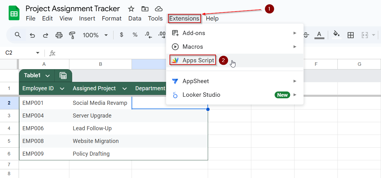
➤ Replace the default code with the script below:
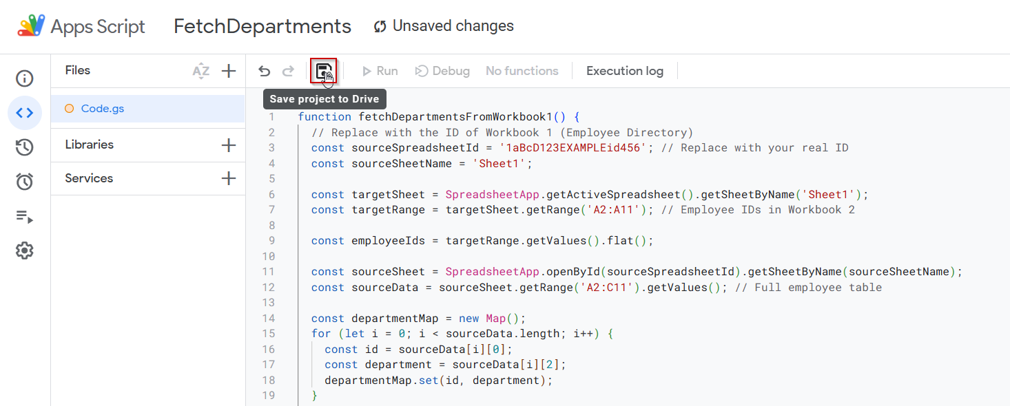
function fetchDepartmentsFromWorkbook1() {
  // Replace with the ID of Workbook 1 (Employee Directory)
  const sourceSpreadsheetId = '1aBcD123EXAMPLEid456'; // Replace with your real ID
  const sourceSheetName = 'Sheet1';
  const targetSheet = SpreadsheetApp.getActiveSpreadsheet().getSheetByName('Sheet1');
  const targetRange = targetSheet.getRange('A2:A11'); // Employee IDs in Workbook 2
  const employeeIds = targetRange.getValues().flat();
  const sourceSheet = SpreadsheetApp.openById(sourceSpreadsheetId).getSheetByName(sourceSheetName);
  const sourceData = sourceSheet.getRange('A2:C11').getValues(); // Full employee table
  const departmentMap = new Map();
  for (let i = 0; i < sourceData.length; i++) {
    const id = sourceData[i][0];
    const department = sourceData[i][2];
    departmentMap.set(id, department);
  }
  for (let i = 0; i < employeeIds.length; i++) {
    const empId = employeeIds[i];
    const department = departmentMap.get(empId) || '';
    targetSheet.getRange(i + 2, 3).setValue(department); // Column C
  }
}
In the script, replace 1aBcD123EXAMPLEid456 with your source file ID.
➤ Click the floppy disk icon or press Ctrl + S to save the script. Name your project something like “FetchDepartments”
➤ Click the Run button
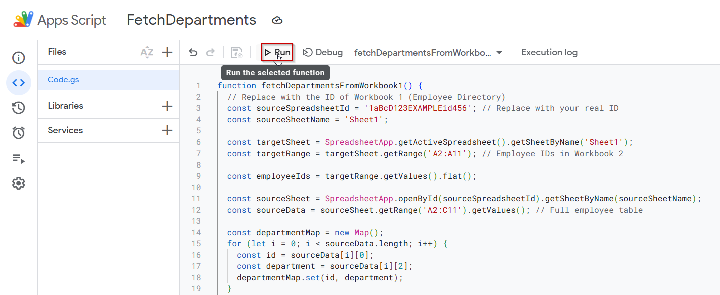
➤ Grant permissions when prompted (only the first time)
The script will loop through each Employee ID in Workbook 2’s Column A and populate Column C with the correct Department from Workbook 1.
Frequently Asked Questions
How do I dynamically pull data from one Google Sheet to another?
You can use the IMPORTRANGE function with VLOOKUP to dynamically fetch data. Simply connect the two sheets with the correct sharing permissions and use Employee ID or another unique value to look up data.
Why do I get a #REF! error when using IMPORTRANGE?
This happens if access hasn’t been granted yet between the two sheets. Click the “Allow access” button that appears once, and the connection will be established permanently unless permissions change.
Can I use IMPORTRANGE with other functions like VLOOKUP or INDEX-MATCH?
Yes, you can combine the IMPORTRANGE function with the VLOOKUP function, INDEX, MATCH, and FILTER. These combinations are especially helpful when you’re referencing data based on unique identifiers or structured datasets.
What’s the best way to fetch specific columns from another workbook?
Use the IMPORTRANGE function to import the desired range (e.g., “Sheet1!A:C“), then apply a lookup function to target a specific column. This is efficient and keeps your destination sheet dynamic and clean.
Why is my Google Apps Script giving a permission error with openById()?
This usually happens because the target script doesn’t have access to the source sheet. Make sure the source sheet is shared with the script owner’s account or is set to “Anyone with the link can view.”
Wrapping Up
Pulling data dynamically between Google Sheets workbooks can significantly streamline multi-sheet workflows, especially when tracking employee details, syncing reports, or consolidating project data. Whether you use the reliable IMPORTRANGE and VLOOKUP functions combo or automate the process with Apps Script, each method offers a way to keep your destination sheet updated without manual copying.
Remember that properly sharing permissions is essential for any method to work smoothly. Once your sheets are connected, updates in one will reflect in the other, saving you time and reducing errors.