When working across multiple spreadsheets, you may need to pull data from a cell in a different Google Sheets file, commonly referred to as referencing another workbook. This is useful for creating dashboards, consolidating reports, or keeping master trackers in sync.
In this article, we’ll show you how to reference a cell from another workbook in Google Sheets using the IMPORTRANGE function, with step-by-step guidance and a sample dataset.
Steps to reference a cell from another workbook in Google Sheets using IMPORTRANGE:
➤ Open the source workbook and note the sheet name and cell you want to reference (e.g., Sheet1!B2)
➤ Update the permission of the Sheet and give edit access to anyone with the link.
➤ In the destination workbook, click the cell where you want the imported data to appear
➤ Enter the formula: =IMPORTRANGE(“source-spreadsheet-URL”, “Sheet1!B2”)
➤ Press Enter, and it will be referenced.
Reference a Cell from Another Workbook Using the IMPORTRANGE Function
The most reliable way to reference a cell from a different Google Sheet is with the IMPORTRANGE function. This allows you to link between two completely separate spreadsheets.
We’ll use two files:
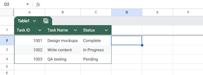
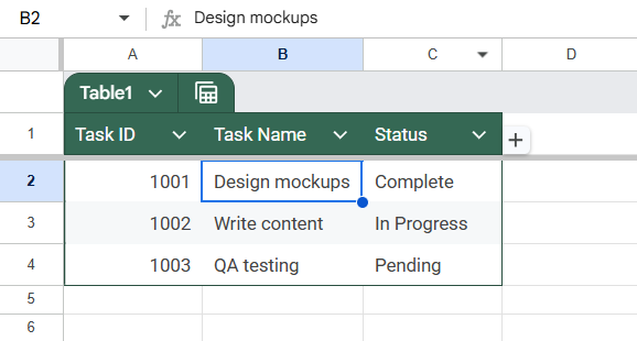
- Source Workbook: Contains a dataset of tasks
- Destination Workbook: A dashboard where we want to reference the tasks from the source.
Let’s say we want to pull cell B2 from Sheet1 of the source file and link it to a cell in the destination workbook.
Steps:
➤ Open your source workbook. This is the Google Sheet that contains the data you want to reference.
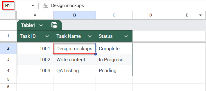
➤ Locate the exact cell you want to pull from. For example, let’s say it’s cell B2 in Sheet1 of the source file.
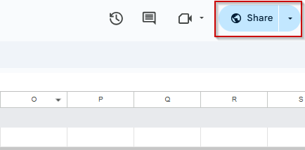
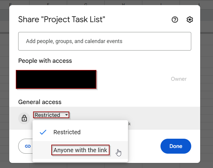
➤ Go to your screen’s top right corner and click the Share button.
➤ Click on Restricted, and then choose Anyone with the link from the drop-down list.
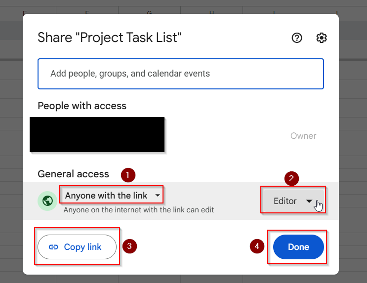
➤ Once you have opened access for everyone with a link. Click on Viewer access and change it to Editor.
➤ Once Access has been updated the popup tablet should look like the screenshot below. Simply Click on Copy link to get the URL of the sheet and then click on Done.
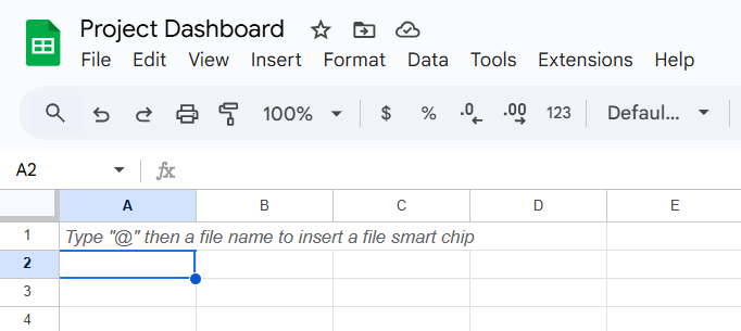
➤ In your destination workbook, open the sheet where you want the data to appear.
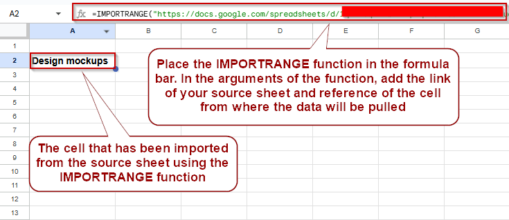
➤ Click on the cell where the referenced data should go. For this example, we’ll use cell A2.
➤ Enter the following formula into the cell. Make sure to change the link in the formula with the link you copied above.
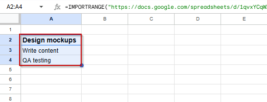
=IMPORTRANGE(“https://docs.google.com/spreadsheets/d/ENTERYOURLINK”, “Sheet1!B2”)

You only need the URL portion up to /edit. You can remove anything after it.
➤ Press Enter on your keyboard.
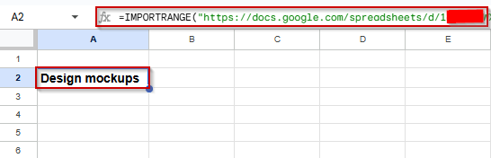
The value from Sheet1!B2 in the source sheet will appear in the destination cell (A1 in this example).
➤ If you want to reference additional cells or even an entire range, you can use the formula below and drag it down to other cells.
=IMPORTRANGE(“URL”, “Sheet1!B2:B4”)
This will import the values from cells B2 through B4 in the source sheet.
Use Google Apps Script to Reference a Cell in Another Workbook in Google Sheets
Google Apps Script is a powerful method if you want to go beyond basic formulas and add more flexibility or automation to referencing data between workbooks. Unlike the IMPORTRANGE function, Apps Script allows you to write custom functions, control how and when data is pulled, and even apply logic before displaying values.
We’ll use the same dataset for consistency.
Steps:
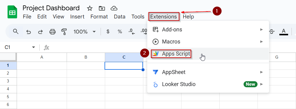
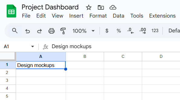
➤ Open the Target Sheet (Project Dashboard), where you want to pull the data.
➤ In the menu, click on Extensions >> Apps Script.
➤ This opens the script editor. Delete any existing placeholder code in the editor.
➤ Paste the following custom function into the script editor:
function copyStatusToCell() {
  var sourceSpreadsheet = SpreadsheetApp.openById("1aBcD123EXAMPLEid456");
  var sourceSheet = sourceSpreadsheet.getSheetByName("Sheet1");
  var value = sourceSheet.getRange("B2").getValue();
  var destinationSheet = SpreadsheetApp.getActiveSpreadsheet().getSheetByName("Sheet1");
  destinationSheet.getRange("A1").setValue(value);
}
Replace 1aBcD123EXAMPLEid456 with the actual Sheet ID of your Project Tracker. This ID comes from the URL of your source file:
https://docs.google.com/spreadsheets/d/1aBcD123EXAMPLEid456/edit
The script above will pull cell B2 from the source file and transfer it to cell A1 in the destination file.
➤ Once updated, click the floppy disk icon to save the script and give your project a name (e.g., ProjectStatusReference).

➤ Run the script and assign the required permissions from your Google account.
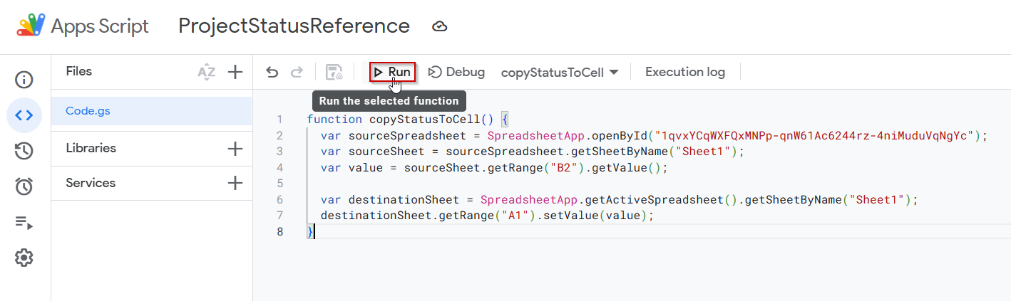
➤ Once the script runs, you can return to your target sheet and notice that the cell B2 we wanted to reference from the source sheet is already there in A1.
Frequently Asked Questions
How do I reference a cell from another Google Sheet?
Use the IMPORTRANGE function with the source sheet’s URL and range,
➤ Use the formula: =IMPORTRANGE(“sheet_url”, “Sheet1!A1”)
➤ Click “Allow access” when prompted.
Why does IMPORTRANGE show a #REF! error?
This usually happens when permission hasn’t been granted. Click “Allow access” when prompted, or check if the source sheet is shared with the current user’s Google account.
Is it possible to reference a sheet in another workbook using a script?
Yes, you can use Apps Script with openById function and getSheetByName function, but the script must run with authorization and correct permissions, especially in personal vs. workspace accounts.
What’s the difference between IMPORTRANGE and Apps Script for referencing cells?
The IMPORTRANGE function is formula-based and easy for most use cases. Apps Script gives more control and logic but requires permissions and scripting knowledge for setup and maintenance.
Wrapping Up
Referencing a cell from another Google Sheets workbook is a powerful feature that enables real-time data syncing across files. Whether you use the straightforward IMPORTRANGE function or set up a more advanced App Script connection, both methods allow you to streamline multi-sheet workflows and avoid manual copy-pasting.
For most users, the IMPORTRANGE function is quick, reliable, and works well for both individual cells and ranges. Google Apps Script offers a more flexible but technical solution for those needing automation, customization, or logic-based imports.