How to Add Days to a Date in Google Sheets (4 Quick Methods)

When working with schedules, deadlines, or tracking systems, you often need to calculate future dates by adding a number of days to a given date. Google Sheets makes this incredibly easy with basic arithmetic and built-in functions.

In this article, we’ll show you multiple ways to add days to a date in Google Sheets using formulas like addition, EDATE, and WORKDAY functions. We’ll also use a realistic dataset to make each method relatable and easy to follow.

If you’re managing employee leave records, one of the most common tasks is figuring out when each person is expected to return to work. The easiest and most direct way to do this in Google Sheets is by adding the number of leave days to the start date using a simple addition formula.

This method is perfect when working with a basic leave tracker, where each row represents an employee’s leave request, including their name, start date, and number of leave days.

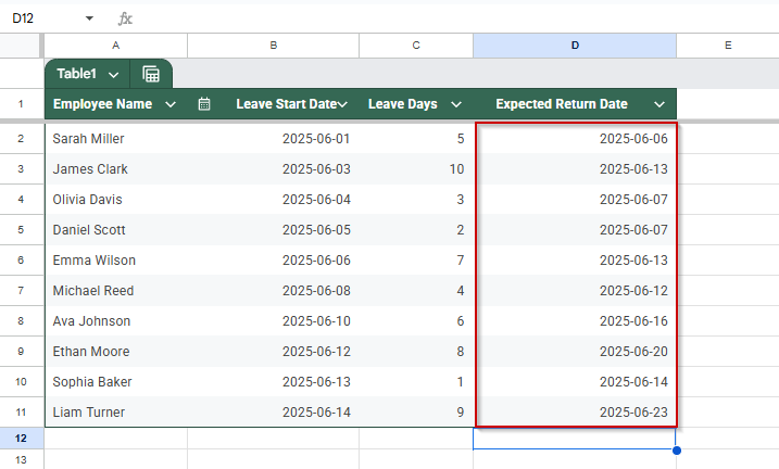
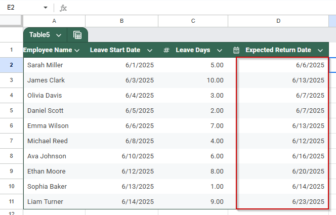
We will be using the following dataset for this article:

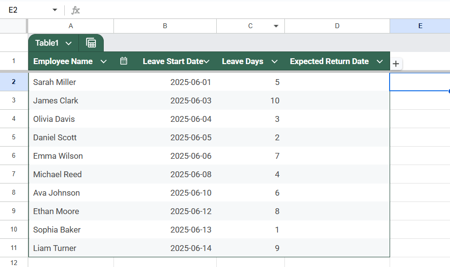
We’ll calculate the Expected Return Date by adding the Leave Days (Column C) to the Leave Start Date (Column B).

Steps:

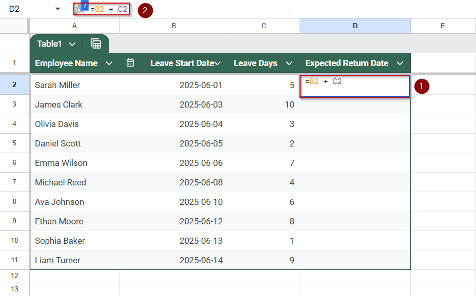
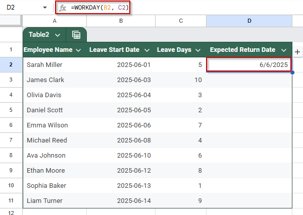
➤ Click on cell D2, where the return date for Sarah Miller will appear.
➤ Enter the formula:

➤ Press Enter. You might see a number like 45815, which is Google Sheets’ internal date serial number.

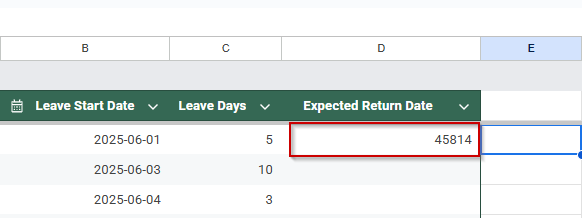
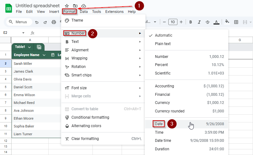
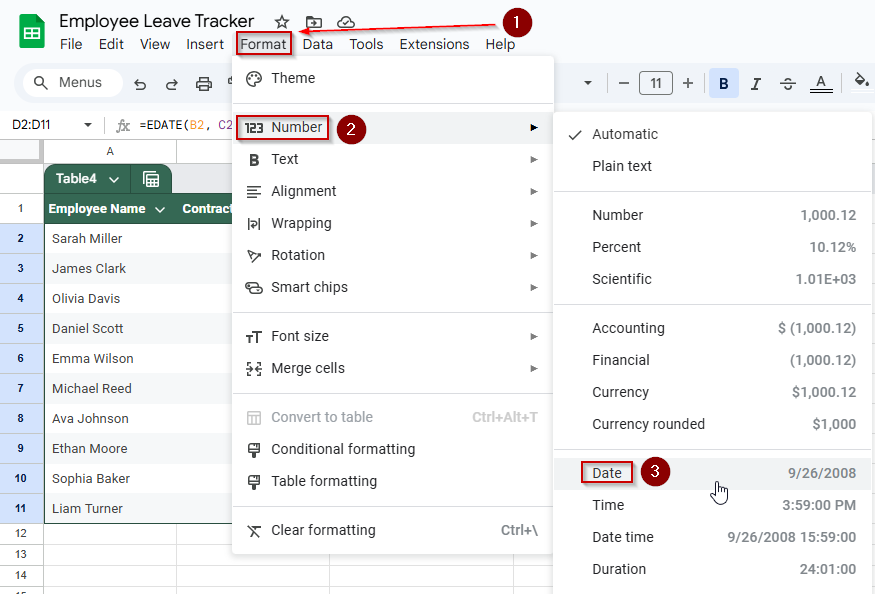
➤ To format it correctly, go to Format >> Number >> Date to convert the serial number into a readable date (like 2025-06-06).

➤ Drag the fill handle down from D2 to D11 to apply the formula to the rest of the employees.

Each employee’s return date is now calculated based on their start date and leave duration.

When calculating dates, especially in business settings, it’s often necessary to exclude weekends. That’s where the WORKDAY function comes in. It lets you add working days to a date, skipping Saturdays and Sundays by default.

This method is great for HR teams, project planners, or anyone managing schedules where only weekdays are counted.

Steps:

➤ Click on cell D2 (or wherever your “Expected Return Date” column starts).
➤ Type the following formula:

➤ Press Enter.

This calculates the return date while skipping weekends.

➤ Use the fill handle to drag the formula down from D2 to D11.

Now, all your return dates will fall on weekdays, making the schedule more practical for typical business operations.

➤ If your company has custom holidays, you can include them in a separate sheet and pass that as the third argument in your leave tracker.

➤ This would be the formula in case you want to add Holidays,

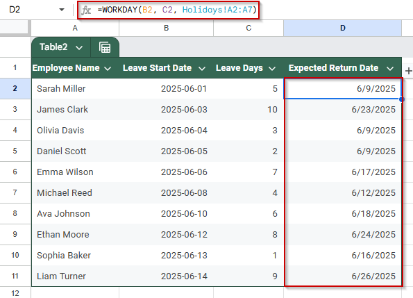
This adds even more precision by excluding public holidays or company shutdowns.

The EDATE function in Google Sheets is used to add (or subtract) a specific number of months to a given date. This is especially useful in HR, finance, or project planning where durations are measured in months instead of days.

Let’s say your company grants fixed-term contracts that last several months, and you want to calculate the contract end date for each employee. This method is how you will achieve that!

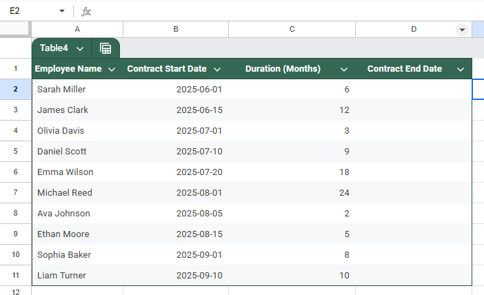
This is the dataset that we will be using for this method.

Steps:

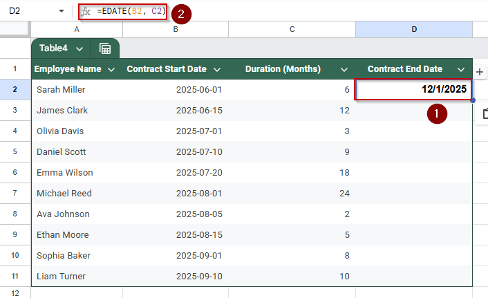
➤ Click on cell D2, where we’ll enter the formula to calculate the contract end date
➤ Enter the formula:

➤ Press Enter. You’ll see the end date appear in D2.

➤ Use the fill handle to drag the formula down through D11 to apply it to all employees.

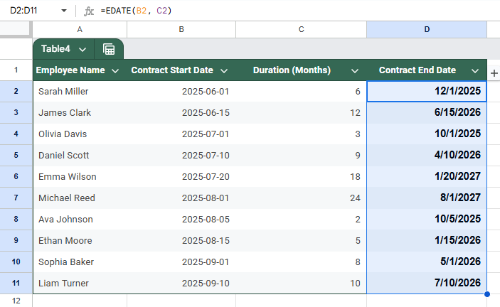
➤ If the result appears as a serial number (e.g., 45321), format the column by going to Format >> Number >> Date to display a readable date format.

If you frequently need to add a number of days to dates across your sheet, for instance, adding leave duration to a start date, Google Apps Script can automate the task. This method processes each row and writes the result in a new column.

Steps:

➤ Open your Google Sheet.
➤ Go to Extensions >> Apps Script.

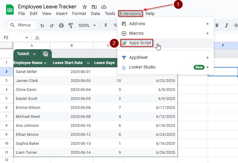
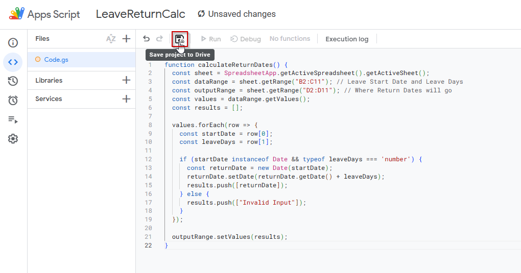
➤ Delete any default code and paste the following:

function calculateExpectedReturnDates() {
  var sheet = SpreadsheetApp.getActiveSpreadsheet().getSheetByName("Sheet1");
  var lastRow = sheet.getLastRow();
  for (var i = 2; i <= lastRow; i++) {
    var startDateRaw = sheet.getRange(i, 2).getValue();
    var leaveDaysRaw = sheet.getRange(i, 3).getValue();
    var startDate = new Date(startDateRaw);
    var leaveDays = parseFloat(leaveDaysRaw);
    if (!isNaN(startDate.getTime()) && !isNaN(leaveDays)) {
      var returnDate = new Date(startDate);
      returnDate.setDate(returnDate.getDate() + leaveDays);
      sheet.getRange(i, 4).setValue(returnDate);
    } else {
      sheet.getRange(i, 4).setValue("Invalid input");
    }
  }
}

➤ Save the project by clicking on the floppy disk icon (you can name it something like LeaveReturnCalc).

➤ Click the Run button once. The script might ask for authorization to approve the necessary permissions.

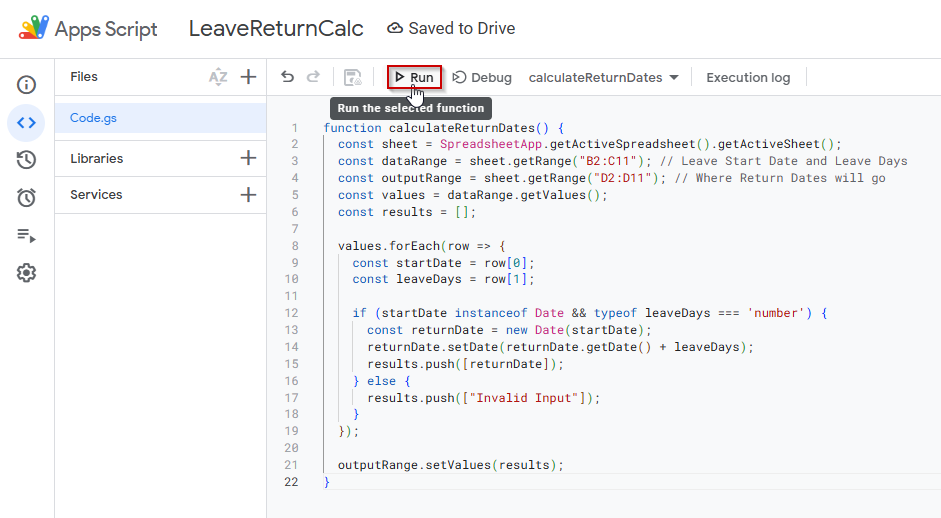
Once run, Column D (Return Date) will be filled in based on the start date and leave days in Columns B and C.

Frequently Asked Questions

How do I add a specific number of days to a date in Google Sheets?

You can simply use the formula =B2 + C2, where B2 is the start date and C2 contains the number of days. Google Sheets automatically handles date arithmetic and returns the correct result.

What if I want to exclude weekends or holidays when adding days to a date?

Use the WORKDAY function: =WORKDAY(B2, C2, Holidays!A2:A10). It skips Saturdays, Sundays, and any holidays you define in a separate range, ensuring more accurate return dates.

Why am I getting “Invalid input” when using an Apps Script to add days to dates?

This usually means your date or number fields are formatted incorrectly. Ensure dates are actual date objects (not text), and your leave days are valid numbers, not blank or text strings.

Can I dynamically calculate return dates in bulk using Google Apps Script?

Yes. A simple script can loop through your rows, read start dates and leave durations, and populate return dates. This is especially useful when dealing with larger datasets or automating HR workflows.

How do I format the return date properly after calculating it in Google Sheets?

After adding days, use Format >> Number >> Date to ensure the cell is recognized as a date. This ensures consistency across the sheet and prevents errors in formulas or data exports.

Wrapping Up

Whether you’re managing employee leave, project deadlines, or personal schedules, Google Sheets makes it easy to calculate future dates by adding days to a start date. With simple formulas like =StartDate + Days or advanced functions like WORKDAY, you can customize date calculations to fit real-world needs, including skipping weekends or custom holidays.

Google Apps Script adds even more flexibility if you’re handling larger datasets or need automation. Choose the best method for your workflow, and let Sheets do the heavy lifting for you.