You often need to extract text between two characters, such as parentheses, brackets, hyphens, or other delimiters. This task is relatively common when working with large datasets. Using the proper format, this task is easy to do.
In this article, we will guide you through the process of extracting text between two characters using various methods. Let’s see a step-by-step guide.
➤ Extracting text between parentheses, Square brackets, and Hyphens follows the same MID and FIND formula.
➤ Using the REGEXEXTRACT function, you can extract text between curly braces.

Extract Text Between Parentheses
This method will show how easily you can extract text between parentheses.
Steps:
➤ Insert an empty adjacent column named City.
➤ In the first row of the column, type the formula:
=MID(A2, FIND(“(“, A2) + 1, FIND(“)”, A2) – FIND(“(“, A2) – 1)
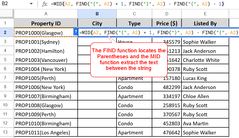
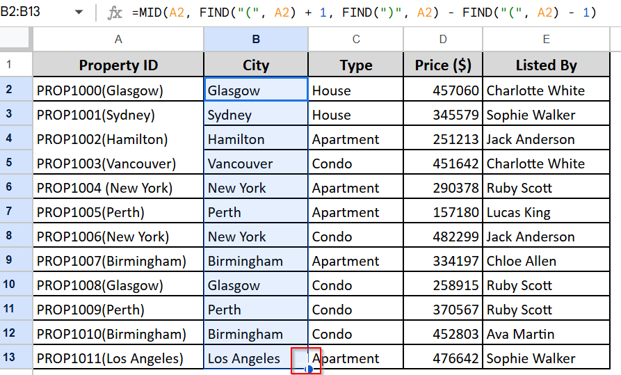
➤ Press Enter, and all the city names will be extracted from the parentheses.
➤ To apply the formula to the whole column, simply drag and drop it to the bottom.
Extract Text Between Square Brackets
Extracting text between square brackets is also similar to the previous one. You just need to make a few minor edits to the formula. Let’s say we want to extract the house type here:
Steps:
➤ Insert an adjacent empty column.
➤ In the first cell of the empty column, insert this formula:
=MID(A2, FIND(“[“, A2) + 1, FIND(“]”, A2) – FIND(“[“, A2) – 1)
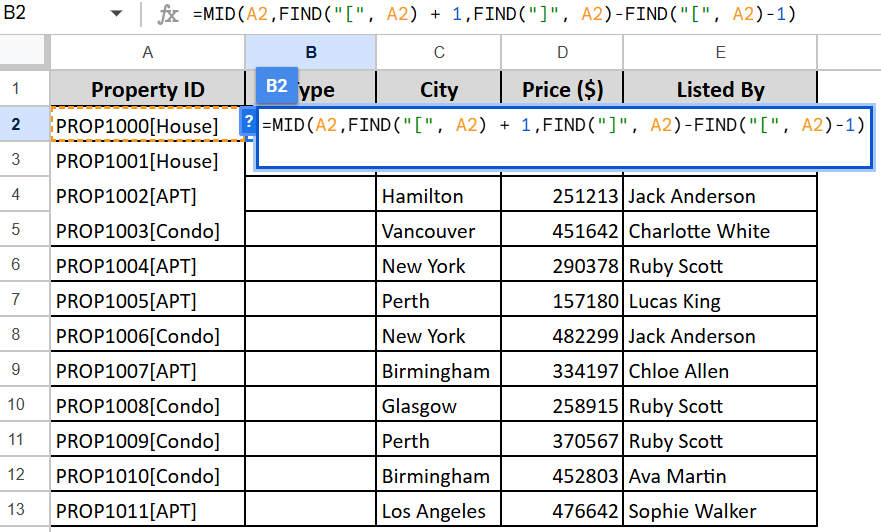
➤ Hit Enter, and you are done!
Extract Text Between Hyphens
The process of extracting text between hyphens also makes use of the same MID and FIND functions. To extract the text between Hyphens, use this formula:
=MID(A2, FIND(“-“, A2) + 1, FIND(“-“, A2, FIND(“-“, A2) + 1) – FIND(“-“, A2) – 1)
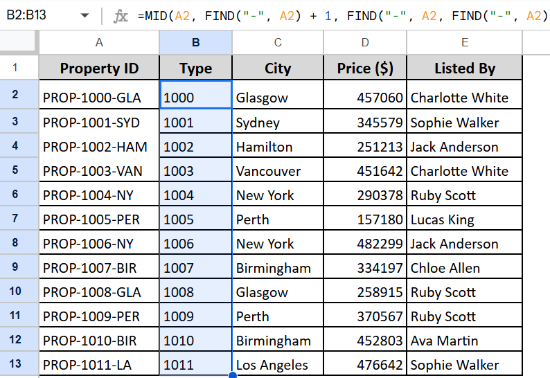
Hit Enter, and all the text between Hyphens is extracted.
Extract Text Between Curly Braces
Extracting text between the curly braces is different than the rest of them. However, there’s a very simple formula to do so:
Steps:
➤ Create a new empty column.
➤ Enter the formula in the first row:
=REGEXEXTRACT(A2, “\{(\d+)\}”)
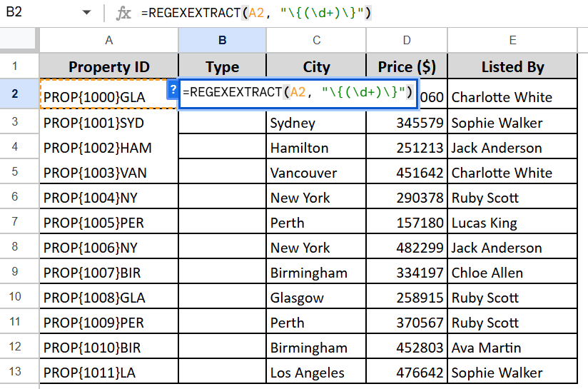
➤ Hit Enter. Drag and drop it to the bottom to fill the row.
Frequently Asked Questions (FAQs)
How do I extract text between characters but ignore case differences?
Use SEARCH() instead of FIND() because SEARCH() is not case-sensitive.
Is it possible to extract text between characters if the delimiter is more than one character?
Yes, but you’ll need to adjust the formula, often using FIND() twice to locate the start and end of the delimiter.
Concluding Words
Using Google Sheets, you can extract texts from all kinds of characters. In this article, we have shown how to extract text between popular characters. If you want to see more or have specific queries, feel free to reach out in the comments. We are eager to hear from you.