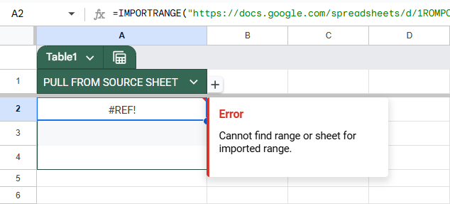
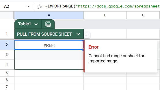
Getting the “Cannot find range or sheet for imported range” error in Google Sheets? You’re not alone. This error pops up most often when using functions like IMPORTRANGE, and it usually means Google Sheets can’t locate the range or sheet you’re trying to pull data from.
This article will guide you through the most common causes of this error and provide step-by-step instructions on how to fix each one. Whether it’s a typo in the sheet name or an issue with permissions, you’ll be able to troubleshoot and resolve the problem quickly.
Steps to correctly use IMPORTRANGE function in Google Sheets:
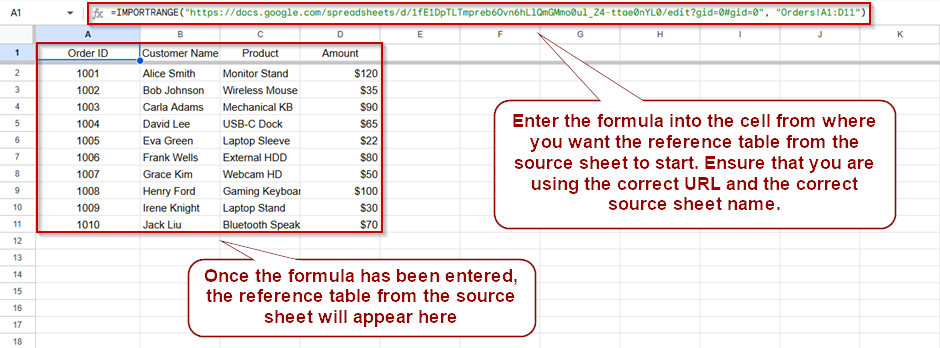
➤Use this template to ensure your formula is correctly structured:
=IMPORTRANGE(“https://docs.google.com/spreadsheets/d/12345abcdXYZ/edit”, “Orders!A1:D11”)
➤ The sheet name (“Orders”) must exist exactly as written in the source file, including spacing and capitalization.
➤ The specified range (A1:D11) must fall within the actual used data in the source sheet.
➤ After entering the formula, you may need to click “Allow Access” to authorize the connection.
➤ Once it works, you can customize the URL and range to suit your own spreadsheet’s structure. Always start with a small, testable range.
Double-Check the Sheet Name
This method helps fix the “Cannot find range or sheet for imported range” error by verifying that the sheet name in your formula exactly matches the tab name in the source spreadsheet. This issue typically occurs due to a typo, a missing space, or incorrect capitalization.
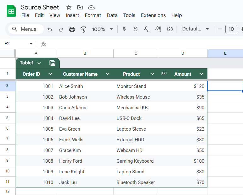
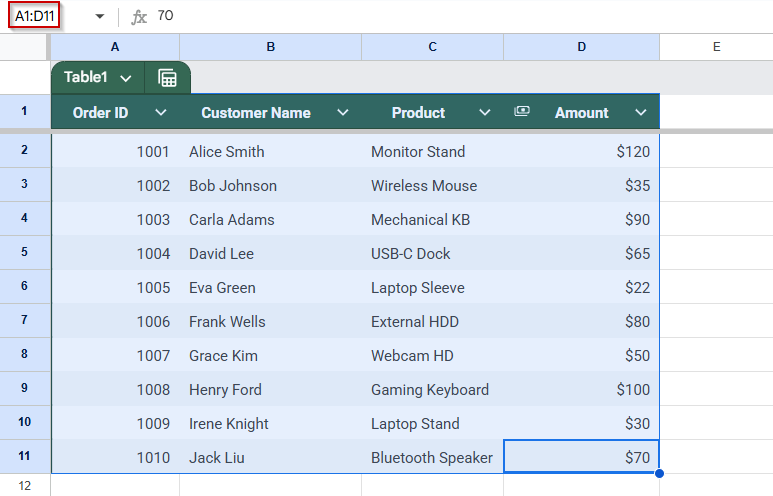
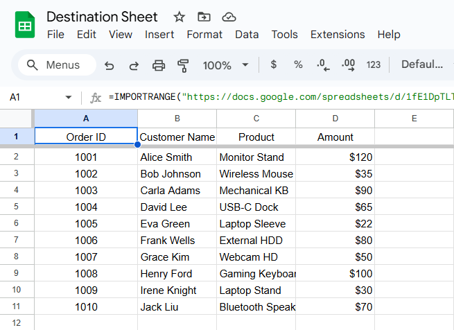
These are the datasets that we will be using to demonstrate the methods:
Source Sheet:
Destination Sheet:

Steps:
➤ Open the source spreadsheet (the file you’re pulling data from).
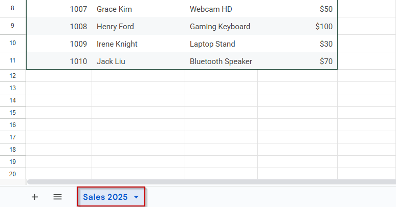
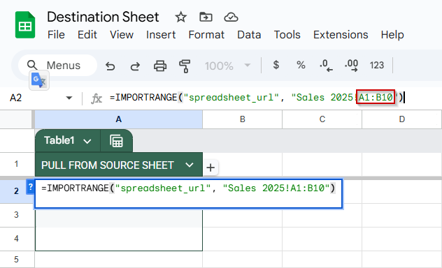
➤ Look at the name of the sheet tab at the bottom (e.g., “Sales 2025”).
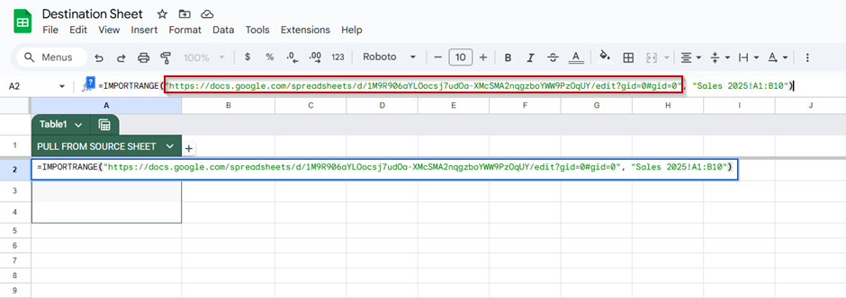
➤ Go to your destination sheet where you’re using the IMPORTRANGE formula.
➤ Make sure the sheet name in the formula matches the tab name exactly, including all spaces and capital letters.
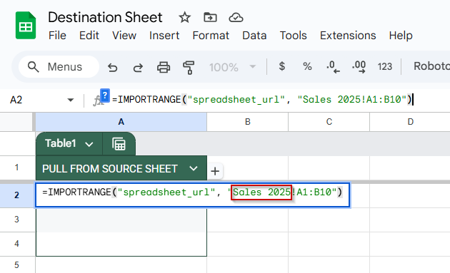
➤ Correct usage:
=IMPORTRANGE(“spreadsheet_url”, “Sales 2025!A1:B10”)
➤ Incorrect usage (missing space or wrong case):
=IMPORTRANGE(“spreadsheet_url”, “sales2025!A1:B10”)
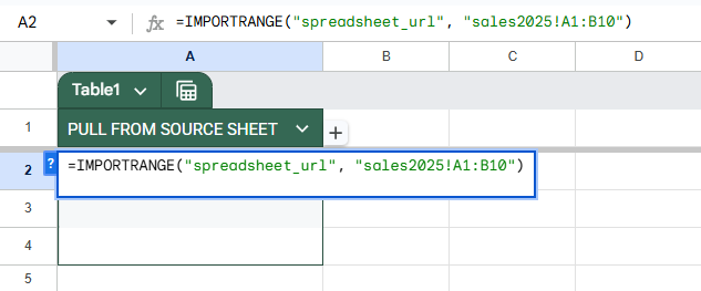
Even a small mismatch will cause the formula to return an error. Always copy the sheet name directly to avoid mistakes.
Make Sure the Range Exists
This method addresses errors caused by referencing a cell range that doesn’t actually exist in the source sheet. If your formula points to a range beyond the available data, Google Sheets can’t retrieve it, resulting in the “Cannot find range or sheet for imported range” error.
Steps:
➤ Open the source spreadsheet and navigate to the sheet you’re importing from.
➤ Review how much data exists, mainly how many rows and columns are in use.
➤ Double-check the range in your IMPORTRANGE formula. Make sure it falls within the actual range of data.
➤ As a test, try changing your formula to a smaller, safe range like “A1:B10” that exists.
➤ Safe test range:
=IMPORTRANGE(“spreadsheet_url”, “Sales 2025!A1:B10”)
➤ Risky range (too large):
=IMPORTRANGE(“spreadsheet_url”, “Sales 2025!A1000:B1200”)
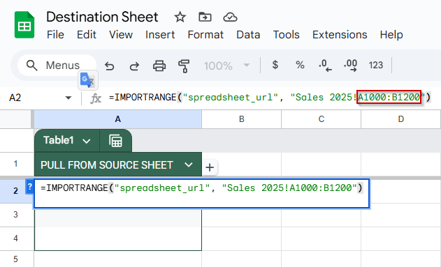
If the target sheet only has 10 rows, the second example will trigger an error. Always confirm that your range selection is valid and contains data.
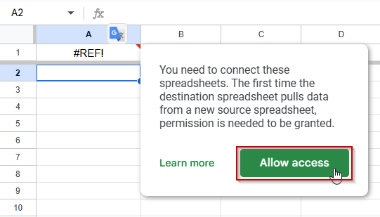
Grant Access to the Source Sheet
Even if your IMPORTRANGE formula is correctly written, it won’t work unless you’ve been granted permission to view the source spreadsheet. Google Sheets needs access to pull the data across files. If access hasn’t been given yet, your formula will return the “Cannot find range or sheet” error. This method shows you how to allow access or request it manually.
Steps:
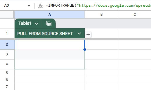
➤ After entering your IMPORTRANGE formula, you’ll see a prompt that says “Allow Access.” Click it.

➤ If the prompt doesn’t appear, open the source spreadsheet directly from the link used in the formula.
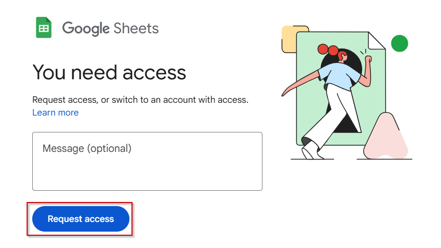
➤ Click “Request access” to ask the owner to share the file with your Google account.
➤ Once access is granted, return to your destination sheet and refresh or re-enter the formula.
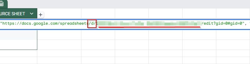
Use the Correct Spreadsheet URL Format
A common mistake is copying only part of the spreadsheet link or pasting the wrong section into your formula. Google Sheets requires the full URL that includes the spreadsheet ID to locate the source file. If the URL is incomplete or incorrect, your formula won’t work no matter what range you specify. This method helps you identify and use the correct link every time.
Steps:
➤ Use the complete Google Sheets URL that looks like this:
https://docs.google.com/spreadsheets/d/SpreadsheetID/edit

➤ Paste it into your formula like so:
=IMPORTRANGE(“https://docs.google.com/spreadsheets/d/1aBcDeFgHiJkLmNoPqRsTuVwXyZ1234567890/edit”, “Sheet1!A1:B10”)
➤ Don’t use shortened links or general URLs like https://docs.google.com.
➤ Make sure the URL contains the /d/ part and the actual spreadsheet ID.
Avoid Quotes Inside Named Ranges While Using IMPORTRANGE Function in Google Sheets
If you’re referencing a named range instead of a standard sheet range, syntax matters. Many users accidentally add extra quotes or use apostrophes, which breaks the formula. IMPORTRANGE requires a clean reference when working with named ranges. This method helps you use them correctly to avoid unnecessary errors.
Steps:
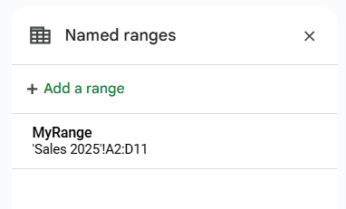
➤ First, confirm the named range exists in the source spreadsheet by going to Data >> Named Ranges.
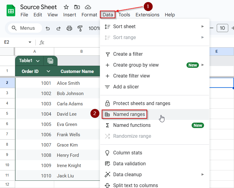
➤ Check on the dashboard to the right to confirm the named range.
➤ In your formula, use it like this:
=IMPORTRANGE(“spreadsheet_url”, “MyRange”)
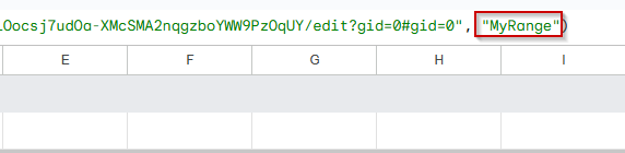
➤ Avoid adding single or double quotes around the named range name (incorrect: “‘MyRange‘”).
➤ Check the spelling and capitalization because it must match the exact name defined in the source file.
Example of a Working IMPORTRANGE Formula in Google Sheets
Sometimes, the best way to troubleshoot is to see a correct formula in action. A well-structured example helps clarify what each part of the function should look like. If you’re unsure about syntax or formatting, start by testing this working version. Once it works, modify it to fit your own spreadsheet.
Steps:
➤Use this formula:
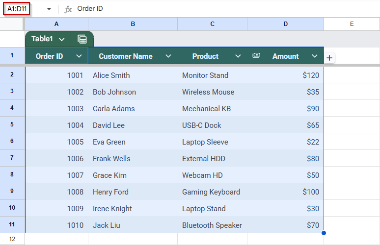
=IMPORTRANGE(“https://docs.google.com/spreadsheets/d/12345abcdXYZ/edit”, “Orders!A1:D11”)
➤ Make sure the sheet name (“Orders“) exists in the source spreadsheet.
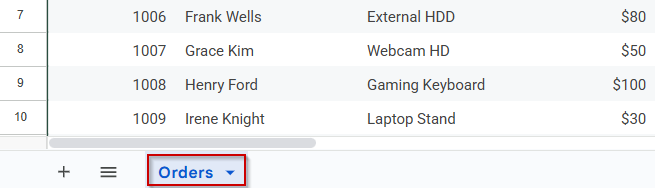
➤ The range (A1:D11) must also exist and contain data.
➤ Access to the source file must be granted when prompted.
➤ Use this as a template and adjust the URL and range to match your specific needs.
Frequently Asked Questions
Can I use IMPORTRANGE across Google accounts?
Yes, you can use IMPORTRANGE across different Google accounts, but you’ll need to ensure the spreadsheet owner has granted your current Google account permission to access the file. Without access, the formula will not work and may trigger the “Cannot find range or sheet” error.
What if the sheet name contains special characters?
If the sheet name includes spaces, symbols, or special characters like &, make sure to wrap the entire name in quotation marks. For example, use “Budget & Sales!A1:C5” so Google Sheets correctly identifies the sheet and avoids formula errors.
Can I use a named range in IMPORTRANGE?
Yes, named ranges are supported in IMPORTRANGE, but they must exist in the source spreadsheet and be typed correctly. Avoid using extra quotes or referencing them like a normal range with Sheet1!. Simply use the named range directly, such as “MyRange“.
Wrapping Up
In this tutorial, we covered simple yet effective ways to fix the “Cannot find range or sheet for imported range” error in Google Sheets. Whether it’s a typo, incorrect range, or access issue, following the steps above will help you resolve it quickly. Once fixed, your IMPORTRANGE function should work without any problems. Feel free to download the practice file and share your feedback.