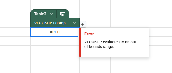
Getting the error “VLOOKUP evaluates to an out of bounds range” in Google Sheets? This issue typically occurs when the column index number in your VLOOKUP formula refers to a column that doesn’t exist within the selected range. It means Google Sheets is being asked to retrieve data from a column that’s beyond the scope of the search range.
This article will guide you through the exact reasons this error appears and show you how to resolve it with step-by-step methods. Whether it’s due to an incorrect column index or a misaligned range, the solutions below will help you fix the error quickly and prevent it in the future.
Steps to correctly use VLOOKUP function in Google Sheets:
➤ Use this template to ensure your formula is correctly structured:
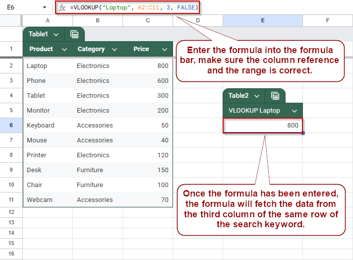
=VLOOKUP(“SearchKeyword”, A2:C11, 2, FALSE)
➤ The lookup range (e.g., A2:C11) must include both the column containing the search key and the column containing the value you want to return.
➤ The column index number must be within the bounds of the lookup range. For a 3-column range, use an index between 1 and 3.
➤ Avoid referencing a column index that exceeds the number of columns in the range. Doing so will trigger an “out of bounds” error.
Double-Check the Column Index Number
This method helps fix the “VLOOKUP evaluates to an out of bounds range” error by confirming that the column number you’re referencing actually exists within your lookup range. This error typically appears when the column index in your VLOOKUP formula is higher than the number of columns in the selected range.
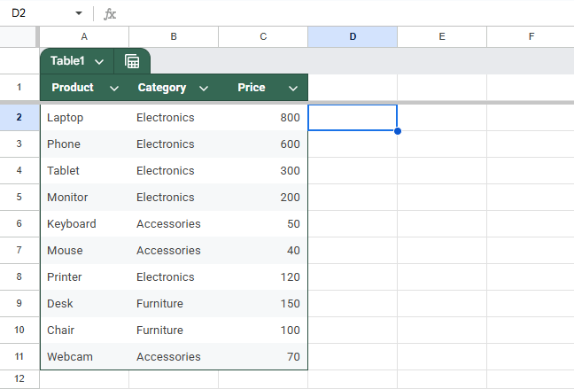
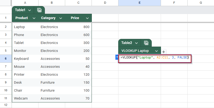
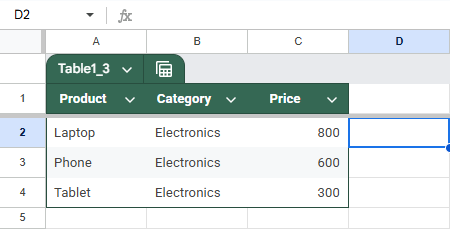
This is the dataset that we will be using to demonstrate the methods:
Steps:
➤ Go to the sheet where you’re using the VLOOKUP function to reference the product data.
➤ Check the range used in your formula. For example:
=VLOOKUP(“Laptop”, A2:B11, 3, FALSE)

➤ In this case, even though the dataset includes three columns, the selected range A2:B11 only includes two: Product and Category.
➤ Because the formula asks for column 3, but the range only includes two columns, this will return the “evaluates to an out of bounds range” error.
➤ To fix it, expand the lookup range to include all the necessary columns:
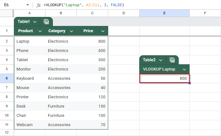
=VLOOKUP(“Laptop”, A2:C11, 3, FALSE)
➤ Always make sure that the column index number you provide is less than or equal to the number of columns in your lookup range, not just in the dataset overall.
Using the correct range will ensure your VLOOKUP formula works without triggering out-of-bounds errors.
Use the COLUMNS Function to Set the Column Index
This method helps fix the “VLOOKUP evaluates to an out of bounds range” error by dynamically calculating the correct column index number using the COLUMNS function. This is especially useful if your lookup range might change in width later. It ensures that your formula always uses a valid column index and prevents out-of-bounds errors.
Steps:
➤ First, determine the number of columns in your lookup range using the COLUMNS function. For example:
=COLUMNS(A2:C11)
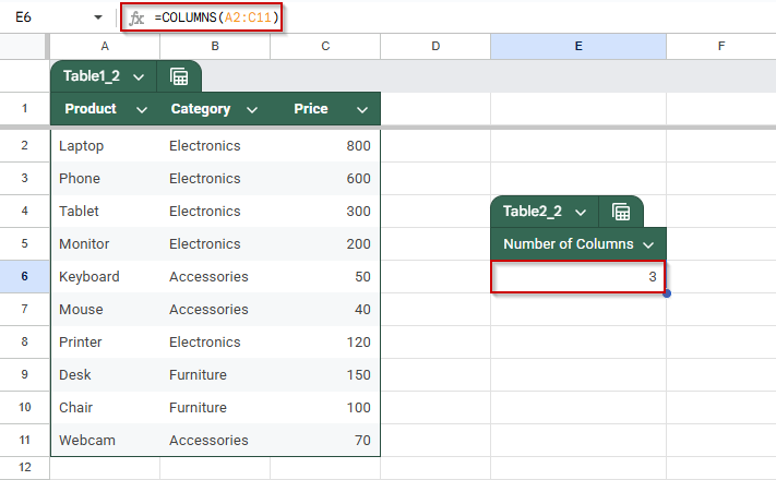
This will return 3, which means the maximum column index you can safely use in a VLOOKUP with this range is 3.
➤ Instead of hardcoding the column index, apply the COLUMNS function directly in your VLOOKUP formula like this:
=VLOOKUP(“Phone”, A2:C11, COLUMNS(A2:C2), FALSE)
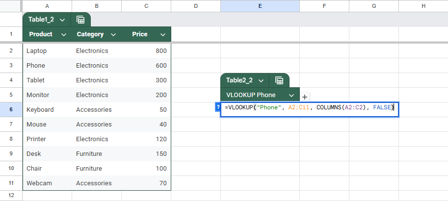
This approach ensures the column index adjusts automatically with changes to the range’s width. If you later expand or reduce the range, your formula stays valid and avoids out-of-bounds errors.

Using the COLUMNS function is a reliable way to future-proof your VLOOKUP formulas, especially in dynamic datasets.
Test Your Range with a Simpler Example
This method helps identify the cause of the “VLOOKUP evaluates to an out of bounds range” error by isolating your formula in a simplified, controlled dataset. Using a smaller table makes it easier to test different column index values and confirm what’s causing the error.
Steps:
➤ Start with a basic three-column table with three rows of data.
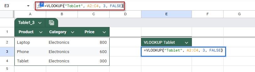
➤ Test your VLOOKUP formula with a correct column index that exists within the range:
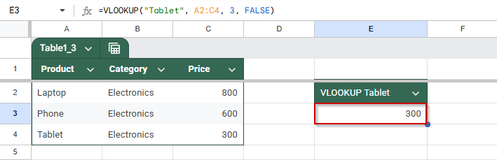
=VLOOKUP(“Tablet”, A2:C4, 3, FALSE)
➤ This will return 300, since “Tablet” is found in the first column and the value from the third column is returned.
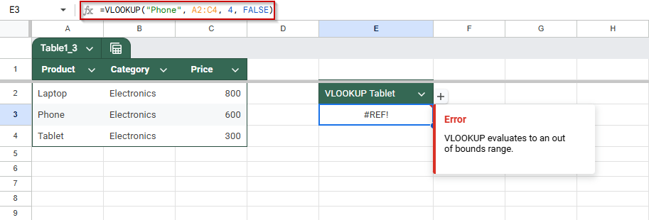
➤ Now test the same formula with an out-of-bounds column index:
=VLOOKUP(“Phone”, A2:C4, 4, FALSE)
➤ This formula will return an error because your range A2:C4 includes only 3 columns, and asking for the 4th column is invalid.
Testing with a simplified range is a quick way to validate your formula structure. Once confirmed, apply the corrected logic back to your main dataset.
Frequently Asked Questions
What does “VLOOKUP evaluates to an out of bounds range” mean?
This error means your VLOOKUP formula is trying to return a value from a column number that doesn’t exist in the lookup range. For example, if your range only spans columns A to B, using a column index of 3 will trigger this error.
How do I know which column index to use in VLOOKUP?
Count the number of columns in your lookup range. The column index in your formula must be between 1 and the total number of columns. You can also use the COLUMNS function to calculate this automatically.
Can I avoid the out-of-bounds error when the range changes?
Yes, by using a dynamic formula with the COLUMNS function, like:
=VLOOKUP(“SearchKey”, A2:C11, COLUMNS(A2:C2), FALSE)
This way, your formula adjusts automatically to the number of columns in the range, preventing out-of-bounds errors.
Wrapping Up
The “VLOOKUP evaluates to an out-of-bounds range” error is caused by a mismatch between the column index number and the size of your selected range. Always make sure your column number is within bounds, and consider using functions like COLUMNS to future-proof your formulas. With a few quick checks, you can eliminate this error and make your VLOOKUP formulas more reliable.