Managing multiple spreadsheets can be tricky, mainly when your data is spread across different files. With the VLOOKUP function, you can automatically fetch matching values from another Google Sheet, like product prices, employee names, or status updates. This eliminates manual copy-paste, reduces errors, and ensures your data always stays up to date.
In this article, we’ll walk through practical ways to use VLOOKUP with data from a separate workbook, using real examples you can follow and customize.
Steps to use VLOOKUP to fetch matching data from another workbook:
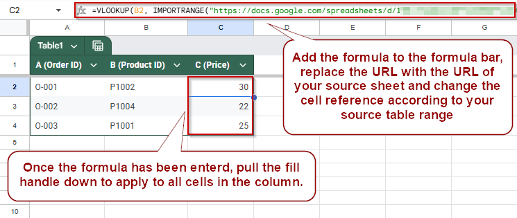
➤ Open the destination sheet (e.g., Order Tracker) and click on cell C2.
➤ Type this formula (replace the URL with your actual source sheet link):
=VLOOKUP(B2, IMPORTRANGE(“https://docs.google.com/spreadsheets/d/abc123XYZ456”, “Sheet1!A2:C6”), 3, FALSE)
➤ IMPORTRANGE pulls columns A–C from the source sheet.
➤ VLOOKUP matches the Product ID from B2 and returns the value in column 3 (Price).
➤ Press Enter. On first use, click Allow Access to connect the sheets.
➤ Drag the formula down to apply it to other rows in the destination sheet.
Basic VLOOKUP Function to Fetch Data Across Workbooks in Google Sheets
When working with related data split across two spreadsheets, such as a product catalog in one and a sales tracker in another, combining VLOOKUP with IMPORTRANGE lets you match values like Product IDs and retrieve corresponding details like prices or categories. This method keeps your sheets connected in real time, ensuring that any updates in the source file are instantly reflected in the destination sheet.
We will use two datasets for this article:
This is the source sheet called “Product Database” from which we will get the values.

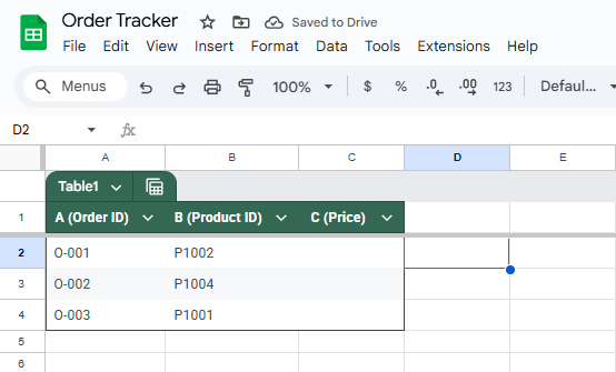
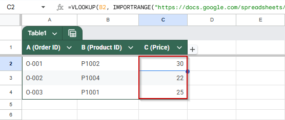
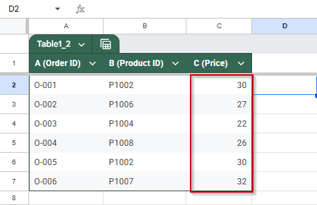
This is the destination sheet called “Order Tracker,” to which the data will be pulled using the VLOOKUP function.
Steps:
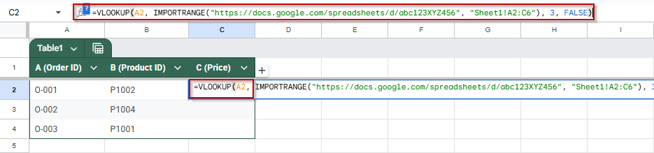
➤ Open the destination sheet (Order Tracker) and click on C2.
➤ Enter the formula (replace the URL with your actual source sheet’s link):
=VLOOKUP(B2, IMPORTRANGE(“https://docs.google.com/spreadsheets/d/abc123XYZ456”, “Sheet1!A2:C6”), 3, FALSE)
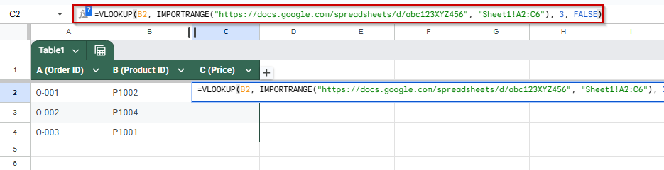
The IMPORTRANGE function fetches columns A–C from the source sheet.. The VLOOKUP function then searches for the Product ID from B2 and returns the value in the 3rd column, the price.
➤ Press Enter.
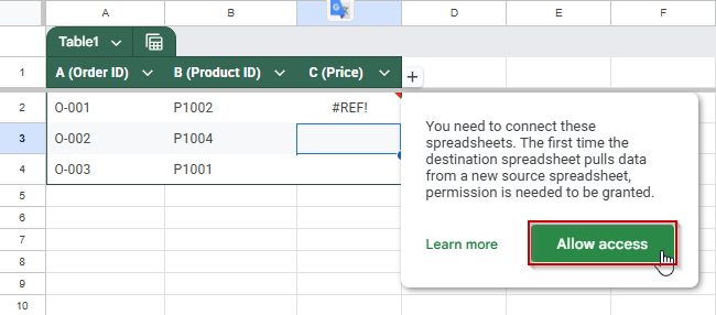
➤ The first time you use IMPORTRANGE, click Allow Access when prompted.
➤ Drag the formula down to apply it to the other rows.
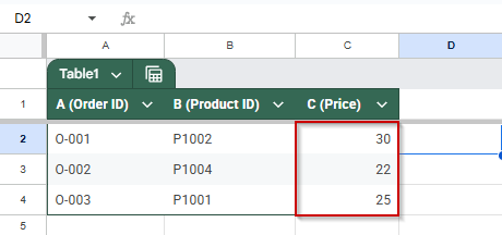
Your prices will now appear dynamically from the source workbook.
VLOOKUP with IMPORTRANGE to Import Named Ranges
If your source spreadsheet uses named ranges, you can reference them directly in your VLOOKUP and IMPORTRANGE formulas. This makes your formula cleaner and easier to manage when dealing with large datasets.
Steps:
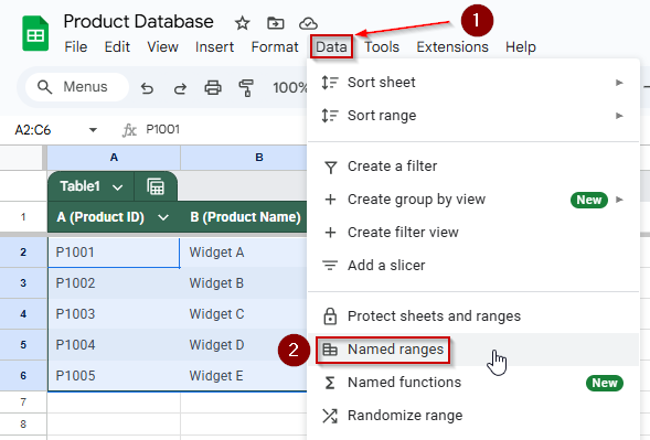
➤ First, open your source sheet.
➤ Select the range you want to name (e.g., A2:C6) and go to Data >> Named ranges.
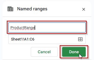
➤ Give the range a name, such as ProductRange.
➤ Now switch to your destination sheet and select the cell where you want the VLOOKUP result to appear.
➤ Paste the formula below:
=VLOOKUP(B2, IMPORTRANGE(“https://docs.google.com/spreadsheets/d/abc123XYZ456”, “Sheet1!A2:C6”), 3, FALSE)
➤ Press Enter and click Allow Access if prompted.
This formula looks up the value in A2, searches for it inside the named range from the external sheet, and returns the second column’s value.
Use VLOOKUP to Pull Data from Two Google Sheets Files at the Same Time
When your data is split across two different Google Sheets (say, “Product Database A” and “Product Database B“), you can combine VLOOKUP, IMPORTRANGE, and IFERROR functions to fetch a value from either file. This is useful when managing distributed product or inventory records.
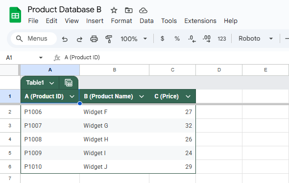
Product Database A is the same source sheet that we used in the past methods; on the other hand, this is what Product Database B looks like:
Steps:
➤ In your destination sheet, click on cell C2.
➤ Type this formula:
=IFERROR(
VLOOKUP(A2, IMPORTRANGE(“https://docs.google.com/spreadsheets/d/FILE_ID_1”, “Sheet1!A:C”), 3, FALSE),
VLOOKUP(A2, IMPORTRANGE(“https://docs.google.com/spreadsheets/d/FILE_ID_2”, “Sheet1!A:C”), 3, FALSE)
)
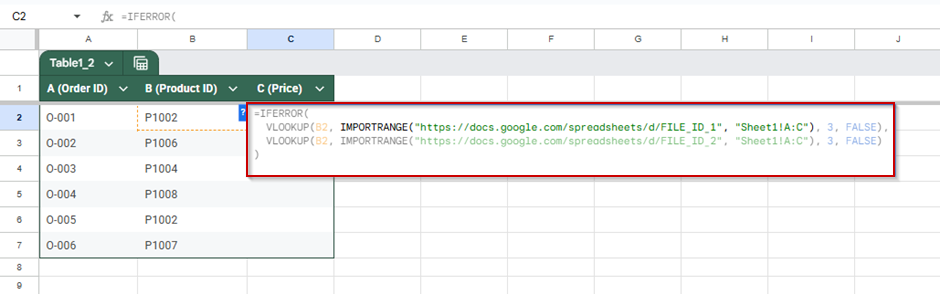
Replace the URLs in the formula with the URL from both your sheets. Each URL in each IMPORTRANGE function. Add more IMPORTRANGE functions if you have more sheets.
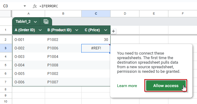
➤ Press Enter. You’ll be prompted to Allow Access the first time you use each IMPORTRANGE link.
➤ Drag the fill handle down to apply the formula to other rows.
The formula checks Product Database A first; if not found, it searches Product Database B.
Frequently Asked Questions
Can VLOOKUP work across different Google Sheets files?
Yes, VLOOKUP can pull data from another spreadsheet using the IMPORTRANGE function to connect to external sheets and retrieve the desired range dynamically.
How do I grant access to another sheet using IMPORTRANGE?
The first time you use IMPORTRANGE, Google Sheets prompts you to click “Allow Access” to link the source sheet. This only needs to be done once.
What happens if the value is not found in the source sheet?
If the value isn’t found, VLOOKUP returns a #N/A error. To avoid this, use IFERROR or search multiple sheets to provide a fallback result.
Can I search multiple external sheets with one VLOOKUP formula?
Yes, by nesting VLOOKUP functions inside IFERROR, you can search across multiple external sheets in order until a match is found or return a default value.
Wrapping Up
Using VLOOKUP across multiple Google Sheets workbooks is a powerful way to keep your data in one place, dynamic, and consistent, without manual copying. By combining VLOOKUP with IMPORTRANGE, you can fetch real-time data from other spreadsheets, including product details, pricing, or employee information. If your data lives in multiple source sheets, nesting functions like IFERROR lets you query them in order.