Conditional formatting in Google Sheets becomes even more powerful when paired with checkboxes. Whether you’re building a task tracker, attendance sheet, or inventory checklist, you can visually change cell formats based on whether a checkbox is checked or not.
In this article, we’ll show you how to apply conditional formatting rules triggered by checkboxes to visually highlight completed tasks, active rows, and more.
Steps to highlight an entire row when a checkbox is checked in Google Sheets:
➤ Select the range A2:B11, which includes your task and due date columns (but not the checkbox column).
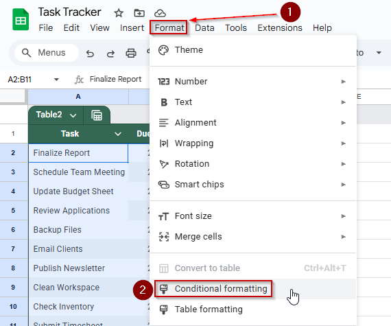
➤ Click on Format in the top menu, then select Conditional formatting.
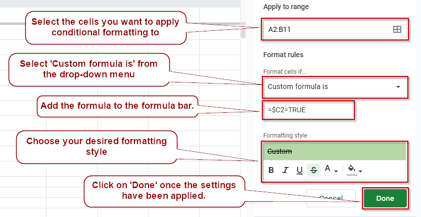
➤ In the Conditional format rules panel, under Format cells if, choose Custom formula is.
➤ Enter the formula: =$C2=TRUE
(This formula checks whether the checkbox in Column C for that row is checked.)
➤ Set a formatting style such as light green background and strikethrough to show the task is completed.
➤ Click Done to apply the rule across the selected rows.
Highlight Row When Checkbox Is Checked
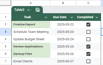
If you’re working with a to-do list or task manager in Google Sheets, using checkboxes to mark tasks as complete is common. You can take it a step further by automatically highlighting an entire row when its checkbox is checked. This improves visibility and helps you quickly spot completed items in your sheet.
We will be using the task tracker below to demonstrate the methods to you:

Steps:
➤ Select the range A2:B11. This should cover the cells that contain task details and due dates (excluding the checkbox column).
➤ Go to the top menu and click Format, then choose Conditional formatting.
➤ The Conditional format rules panel will appear on the right. Under the dropdown labeled Format cells if, choose Custom formula is.
➤ In the formula field, type:=$C2=TRUE
(This assumes the checkboxes are in Column C and you’re starting from row 2. Adjust the formula if your setup is different.)
➤ Set your formatting style. For example, choose a light green fill and enable strikethrough text to indicate the task is complete.
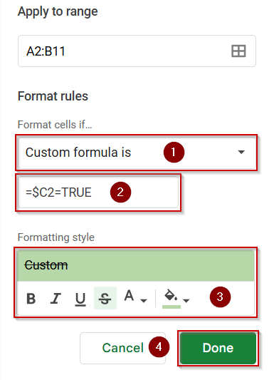
➤ Click Done to apply the rule.
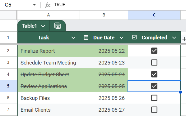
Now, whenever a checkbox is selected in Column C, the entire row from Columns A and B will automatically be formatted with your chosen style. This makes it easy to visually separate completed tasks from pending ones.
Highlighting Due Dates of Incomplete Tasks
When managing tasks in Google Sheets, it’s helpful to draw attention to approaching or overdue items that haven’t been completed yet. With checkboxes in place, you can set up conditional formatting that highlights the due dates of any task where the checkbox remains unchecked.
This method allows you to instantly identify pending items by emphasizing their due dates, making it easier to prioritize your workload and stay on top of deadlines.
Steps:
➤ Select the range B2:B6, which contains your due dates.
➤ Go to the top menu and click Format >> Conditional formatting.

➤ In the Conditional format rules panel, under “Format cells if”, choose Custom formula is.
➤ Enter the formula:
=$C2=FALSE
➤ This formula checks if the corresponding checkbox in Column C is unchecked.
➤ Choose a formatting style, such as red text, bold font, or a light red background, to highlight incomplete tasks.

➤ Click Done to apply the rule.
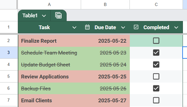
The due dates for any tasks with unchecked boxes in Column C will now stand out, helping you easily spot what still needs attention.
Automate Checkbox-Based Formatting with Apps Script
If you want the task formatting to happen automatically when a checkbox is checked or unchecked, you can use Google Apps Script. This method is useful when you want the task cell to update without using the regular conditional formatting panel. It’s especially helpful for longer checklists where you want fast, consistent formatting.
Once the script is set up, any time you check a box in Column C, the task name in Column A will update right away. Checked tasks will show a green background and strikethrough text. Unchecked tasks will go back to normal.
Steps:
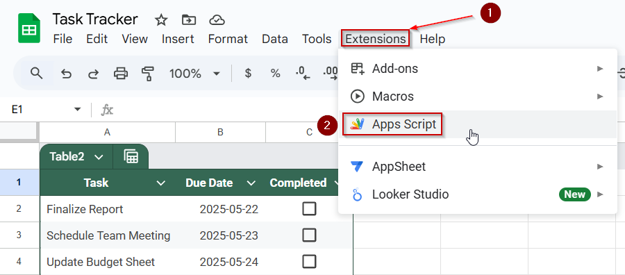
➤ In your Google Sheet, go to Extensions >> Apps Script.
➤ Delete any default code you see in the editor.
➤ Copy and paste the following script:
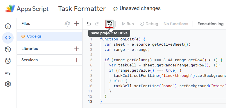
function onEdit(e) {
  var sheet = e.source.getActiveSheet();
  var range = e.range;
  if (range.getColumn() === 3 && range.getRow() > 1) {
    var taskCell = sheet.getRange(range.getRow(), 1);
    if (range.getValue() === true) {
      taskCell.setFontLine("line-through").setBackground("#d9ead3");
    } else {
      taskCell.setFontLine("none").setBackground("white");
    }
  }
}
➤ Save the script by clicking on the floppy disk icon at the top and giving the project a name, such as Task Formatter.
➤ Click the Run button once. You may need to allow permissions the first time.

➤ Go back to your sheet and check a box in Column C.
The task name in Column A will now change automatically. When the box is checked, it turns green and gets a strikethrough. When you uncheck it, the formatting goes back to normal.
Frequently Asked Questions
How do I apply conditional formatting based on a checkbox in Google Sheets?
Use “Custom formula is” in conditional formatting. For example, use =$C2=TRUE to apply a format when the checkbox in column C is checked. Then choose your formatting style and apply it to your target range.
Can I strike through text when a checkbox is checked?
Yes. Select the target text range (like tasks), use conditional formatting with the formula =$C2=TRUE, and apply strikethrough as the format. This helps visually show that the task has been completed without affecting the whole row.
How do I highlight an entire row when a checkbox is ticked?
Select the full row range (like A2:B11), then apply conditional formatting with the formula =$C2=TRUE. This will highlight the entire row when the corresponding checkbox in column C is marked as checked.
Can I use Google Apps Script to automate formatting with checkboxes?
Yes. Google Apps Script can watch for checkbox changes using the onEdit function. When triggered, it can apply formats like strikethrough or background color to specific cells, automating visual feedback for completed tasks or checklists.
Why isn’t my checkbox-based conditional formatting working?
Check that the formula uses absolute references (like $C2), and ensure checkboxes are inserted correctly (Insert >> Checkbox). Also verify your formatting range matches the formula logic and that your checkboxes return TRUE or FALSE values.
Wrapping Up
Checkboxes in Google Sheets are more than just basic tools. When used with conditional formatting, they help make your data more useful and easier to read. You can highlight completed tasks, strike through text, or even use Apps Script to automate formatting. These methods can improve your checklists, task trackers, or project sheets. Use the one that fits your needs and make your spreadsheets work better for you.