When managing data in Google Sheets, highlighting cells based on text in another cell can help you quickly identify patterns, categories, or actions required. Whether you’re reviewing task statuses, sales stages, or student grades, conditional formatting based on adjacent or related cell content makes your data more actionable and readable.
In this article, you’ll learn how to apply conditional formatting to cells when a related cell contains specific text. We’ll use a simple dataset to walk you through step-by-step.
Steps to highlight task cells in Column A based on the status text in Column B:
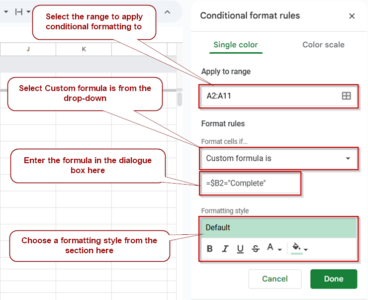
➤ Select the range A2:A11, which includes the task names you want to format.
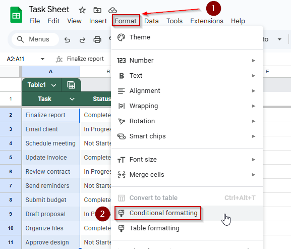
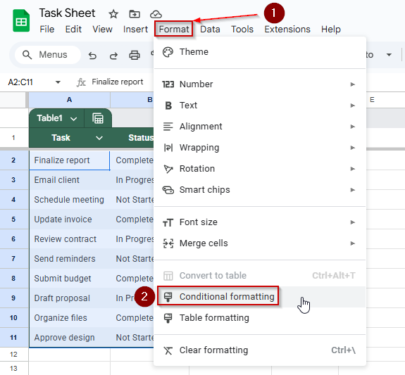
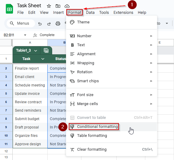
➤ Go to the top menu and click Format >> Conditional formatting.
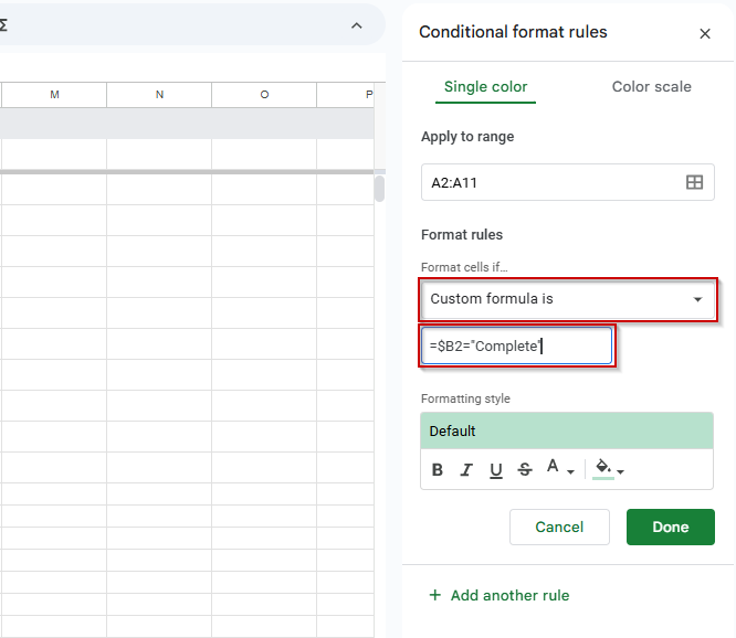
➤ Under Format cells if, choose Custom formula is from the dropdown menu.
➤ In the formula field, enter: =$B2=”Complete”
➤ Choose your formatting style, such as a green background with bold text to highlight completed tasks.
➤ Click Done to apply the rule.
Format Task Cells Based on the Text in Their Corresponding Status Cells in Google Sheets
Sometimes, you may want your task list to visually reflect progress by highlighting tasks based on their status. For instance, if a task is marked “Complete” in Column B, you can automatically highlight the corresponding task in Column A. This method improves clarity and allows you to identify completed tasks by identifying them visually, without manually scanning each row.
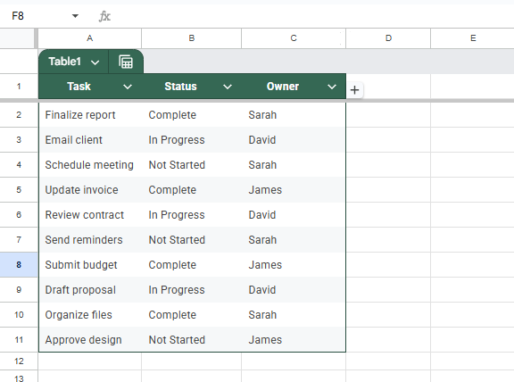
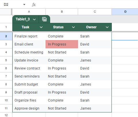
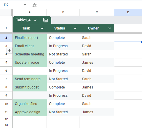
Here’s a sample task management table that we will use for the methods:
Steps:
➤ Select the range A2:A11, which contains your task names. This is the column you want to apply formatting to.
➤ Go to the top menu and click Format >> Conditional formatting. This opens the Conditional format rules panel on the right.
➤ Under the Format cells if dropdown, choose Custom formula is.
➤ In the formula field, type:
=$B2=”Complete”
This checks the value in Column B (Status) for the corresponding row. If the status says “Complete“, the formatting will be applied to the task cell in Column A.
➤ Set your preferred formatting style. For example, to mark the task as complete visually, apply a green fill with bold text.
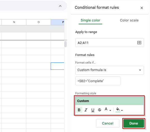
➤ Click Done to finish and apply the rule.
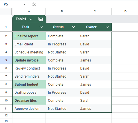
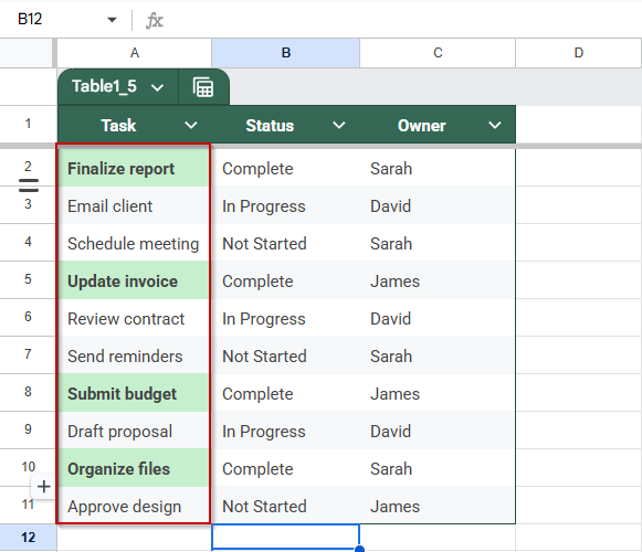
Now, only the task names in Column A that are marked as “Complete” in Column B will be formatted, making it easy to identify finished tasks at a glance.
Highlight Entire Row Based on Text in a Specific Column in Google Sheets
When working with task lists, project trackers, or progress sheets, it can be helpful to emphasize rows based on their status visually. For example, if a task is marked as “In Progress“, you may want the entire row to stand out for quick reference. Using conditional formatting, you can automatically highlight the whole row based on the content of a single column (like the Status column).
Steps:
➤ Select the range A2:C11.
➤ Go to the top menu and click Format >> Conditional formatting.
➤ Under “Format cells if”, choose “Custom formula is”.
➤ In the custom formula field, enter the following:
=$B2=”In Progress”
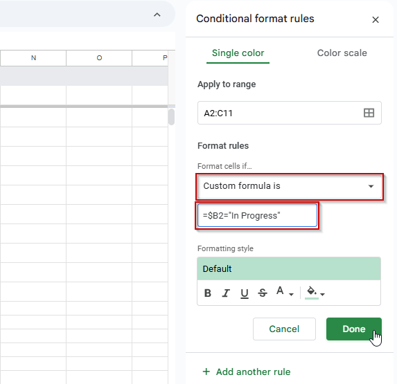
This formula checks whether the current row’s Status column (Column B) contains the text “In Progress”. The dollar sign before B locks the column reference, while the row number stays relative to apply the rule to each row in the range.
➤ Set your formatting style. You can use a yellow background with italic text, or any other style that makes the row stand out visually.

➤ Click “Done” to apply the rule.

Now, any row in your table that has “In Progress” in the Status column will be highlighted according to the style you selected. This makes it easy to scan your sheet and identify ongoing work at a glance.
Apply Conditional Formatting to Status Cells When Tasks Include a Specific Word in Google Sheets
If you want to highlight cells in the Status column based on whether the related Task contains a specific word like “Email,” you can use conditional formatting with a custom formula. This method checks the Task cells for the word and then applies the formatting to the corresponding Status cells, helping you quickly spot tasks related to emails.
Steps:
➤ Select the range B2:B11 (the Status column cells you want to format).
➤ Go to the menu and click Format >> Conditional formatting to open the Conditional Formatting sidebar.
➤ Under Format rules, click the dropdown and select Custom formula is.
➤ In the formula box, enter this formula exactly:
=REGEXMATCH($A2, “Email”)
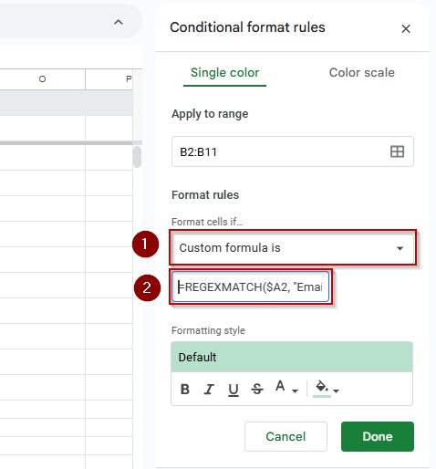
This formula checks if the cell in column A (the Task column) of the current row contains the word “Email“. The dollar sign before A locks the column, while the row number adjusts for each cell in the selected range.
➤ Choose the formatting style you want to apply when the condition is met (for example, set the text color to red).
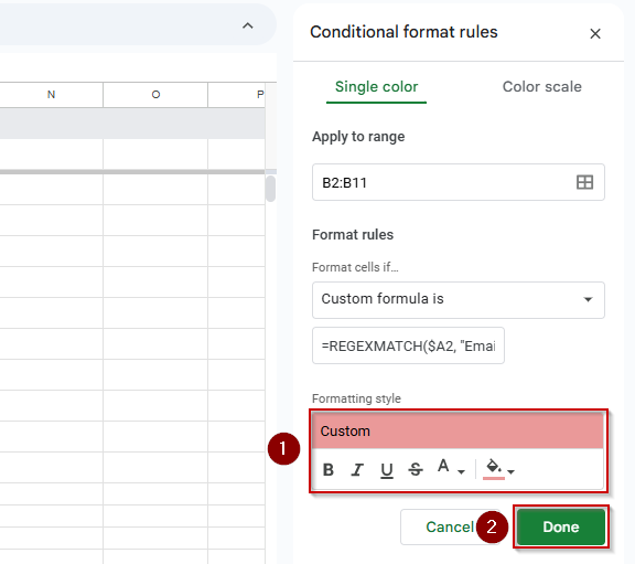
➤ Click Done to apply the rule.
Now, all Status cells in the selected range will be formatted whenever the word “Email” appears in their related task in column A.
Only Format Cells That Have Text Entries in Google Sheets
Suppose you want to apply formatting exclusively to columns containing any text, ignoring empty or non-text cells. In that case, you can use conditional formatting with a custom formula. This technique helps you visually identify all cells with text content, making your data easier to scan.
Steps:
➤ Select the range A2:A11 (the cells in Column A you want to check and highlight).
➤ Go to the menu and click Format >> Conditional formatting to open the Conditional Formatting sidebar.

➤ Under Format rules, click the dropdown menu and select Custom formula is.
➤ In the formula box, enter the following formula exactly:
=ISTEXT(A2)
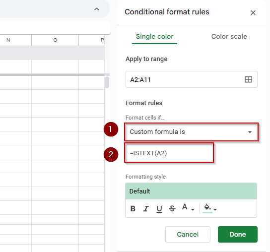
This formula tests if the cell in the current row of Column A contains any text. It returns TRUE for text entries and FALSE for blanks or non-text data.
➤ Choose your preferred formatting style (for example, a background color or font color) to highlight these cells.
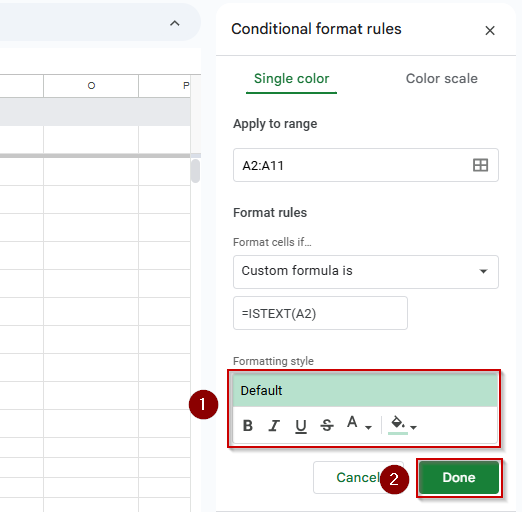
➤ Click Done to apply the rule.
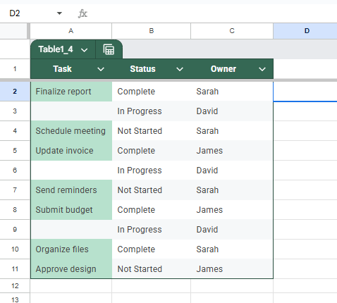
Now, all cells in the selected range that contain text will be highlighted, making it easy to distinguish them from empty or non-text cells.
Automate Conditional Formatting Based on Text Using Apps Script
If you’re managing a large dataset or want to apply conditional formatting automatically without manually setting rules, Apps Script can help. This method highlights a cell in Column A based on the value in Column B.
Steps:
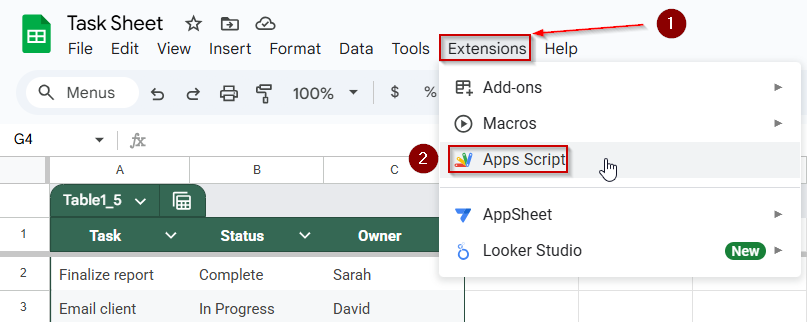
➤ In your Google Sheet, go to Extensions >> Apps Script.
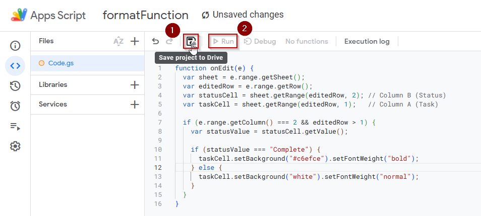
➤ Delete any code in the editor and paste the script below:
function onEdit(e) {
  var sheet = e.range.getSheet();
  var editedRow = e.range.getRow();
  var statusCell = sheet.getRange(editedRow, 2); // Column B (Status)
  var taskCell = sheet.getRange(editedRow, 1);   // Column A (Task)
  if (e.range.getColumn() === 2 && editedRow > 1) {
    var statusValue = statusCell.getValue();
    if (statusValue === "Complete") {
      taskCell.setBackground("#c6efce").setFontWeight("bold");
    } else {
      taskCell.setBackground("white").setFontWeight("normal");
    }
  }
}
➤ Save the script by clicking on the floppy disk icon and authorize it by manually running the function.
Now, every time you update the status in Column B, the task cell in Column A will automatically change its style based on the new value. For example, when the status is set to “Complete“, the task cell gets a green background and bold text.
Frequently Asked Questions
How do I apply conditional formatting based on another cell’s text in Google Sheets?
To do this, use “Custom formula is” in the conditional formatting rules. Reference the other cell using absolute column references like =$B2=”Complete” so it evaluates properly across your selected range.
Can I highlight an entire row based on text in one column?
Yes, select the entire row range (e.g., A2:C11), then use a custom formula like =$B2=”In Progress” in conditional formatting. It will highlight each row where the condition is met.
What if I want to highlight cells based on partial text matches?
Use the SEARCH or REGEXMATCH function in your custom formula. For example: =REGEXMATCH($B2, “Progress”) will match cells that contain “Progress” anywhere in the text.
Can conditional formatting work with text that changes dynamically?
Yes. Conditional formatting updates automatically as the text in the referenced cells changes. For example, if the status changes from “Pending” to “Complete,” formatting will update in real time.
How do I remove conditional formatting once applied?
Go to Format >> Conditional formatting, select the rule in the sidebar, and click Remove rule or Delete. This will remove the formatting from the selected range without affecting your data.
Wrapping Up
Using conditional formatting based on text in another cell can make your Google Sheets much easier to read, understand, and manage. Whether you’re tracking tasks, monitoring project progress, or organizing team responsibilities, these visual cues help you quickly identify what needs attention without scanning every detail. With just a few formulas and clicks, you can automate formatting rules that respond to real-time updates in your data.