If your Google Sheets FILTER function isn’t working as expected, it can be frustrating. Whether it’s returning errors, no results, or incorrect data, the problem usually comes down to range issues, syntax errors, or mismatched filter criteria. Understanding how to set ranges and write criteria correctly is essential to resolving these issues.
This article guides you through the most common Filter issues and provides simple, effective solutions to help you get your data filtering up and running smoothly again.
Steps to use the FILTER function correctly and avoid errors in Google Sheets:
➤ Use this formula structure as a starting point:
=FILTER(A2:C11, B2:B11=”Active”)
➤ Ensure the condition range (e.g., B2:B11) has the same number of rows as the main data range (A2:C11)
➤ Use TRIM or CLEAN if your criteria or data include hidden characters or extra spaces
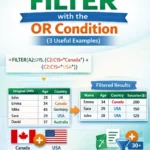
➤ Apply correct logical operators for multiple conditions, such as * for AND and + for OR
➤ Avoid comparing mismatched data types like text to numbers, keep your criteria and data consistent
Solution For Filter Returns #N/A or No Results
One common problem is that the Filter function returns #N/A or shows no results even though matching data exists. This usually happens when the criteria don’t exactly match the data due to typos, extra spaces, or data type mismatches.
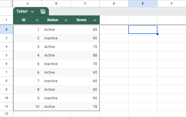
Dataset we’ll use to demonstrate:
Steps:
➤ Verify that the criteria text exactly matches the data (e.g., “Active” with no extra spaces).
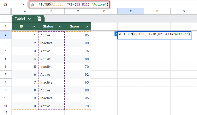
➤ Use the TRIM function to remove unwanted spaces in the requirements or data:
=FILTER(A2:C11, TRIM(B2:B11)=”Active”)
➤ Check the data type; comparing text to numbers or vice versa causes no matches.
➤ Confirm that the range and criteria ranges have the same number of rows.

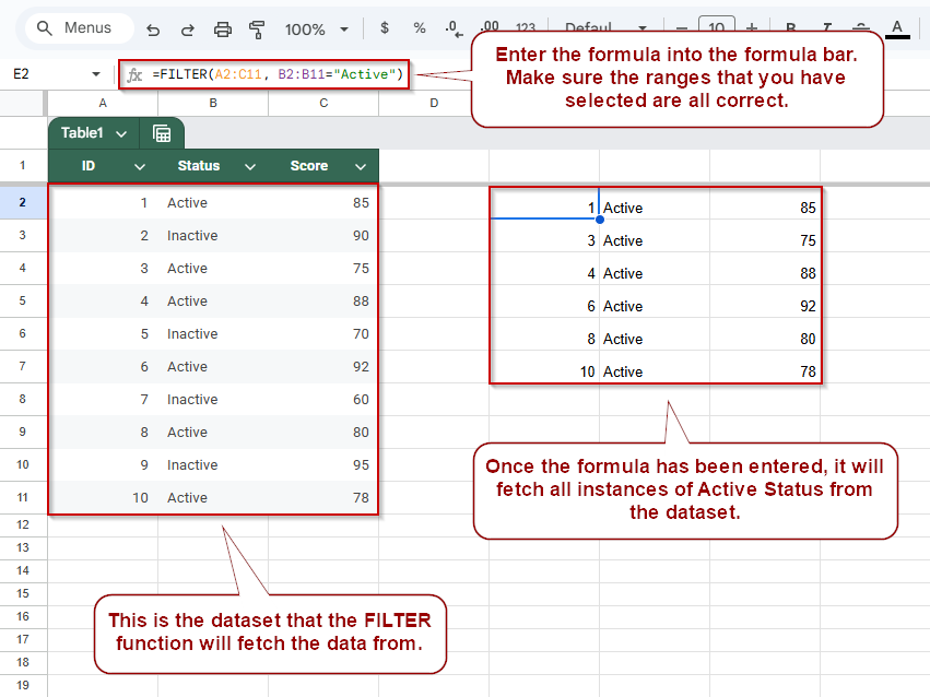
The easiest way to do this is by clicking on the range in the formula bar. This will highlight the formula for you in the Google Sheet. Allowing you to confirm if you selected the correct range or not.
FILTER Returns Wrong or Unexpected Results
If your FILTER formula in Google Sheets returns too many rows, not enough, or results that don’t match your expectations, the issue often lies in how the conditions are written. Using incorrect logic, missing parentheses, or combining incompatible data types can all lead to unexpected behavior.
This method focuses on how to use logical operators like AND and OR properly in your FILTER function to ensure it only includes the rows that actually match your intended criteria.
Steps:
➤ Use proper logical operators depending on the kind of condition you’re applying.
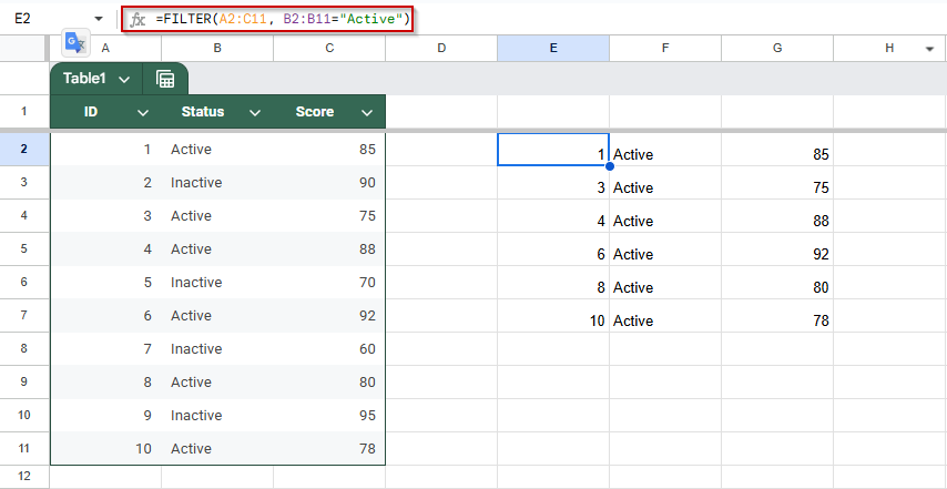
- To filter by one condition (e.g., only rows where Status is “Active”):
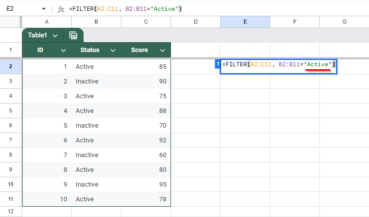
=FILTER(A2:C11, B2:B11=”Active”)
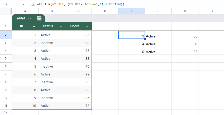
- For multiple conditions using AND logic (e.g., Status is “Active” and Score is greater than 80):
=FILTER(A2:C11, (B2:B11=”Active”)*(C2:C11>80))
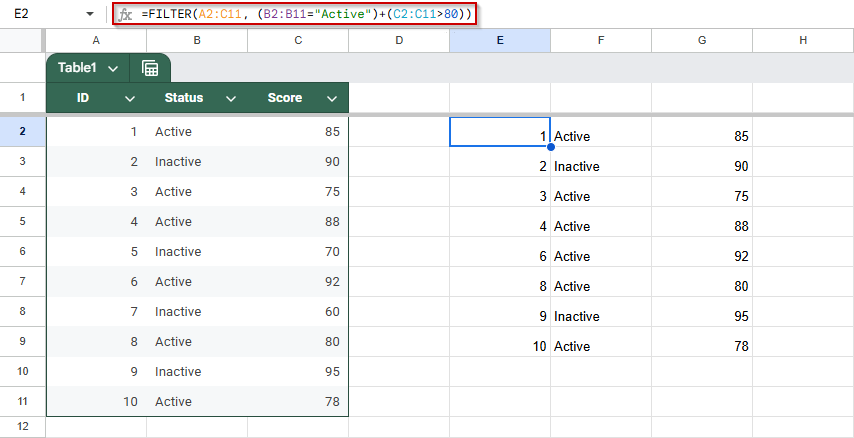
- For OR logic (e.g., Status is “Active” or Score is greater than 80):
=FILTER(A2:C11, (B2:B11=”Active”)+(C2:C11>80))
➤ Always use parentheses to group conditions correctly. Misplaced parentheses can completely change the logic of the formula.
Fix FILTER Range Mismatch Error in Google Sheets
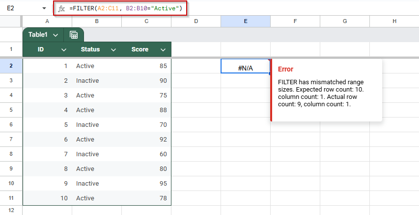
When using the FILTER function in Google Sheets, one common issue is the #REF! error that says: “Array arguments to FILTER are of different size.” This happens when the dimensions of your main data range and your filter condition ranges don’t match. In other words, the number of rows in each range must be the same.
Steps:
➤ Identify your main range (e.g., A2:C11). Count the number of rows; here, it’s 10.
➤ Ensure your condition range (e.g., B2:B11) spans at least 10 rows.
➤ If the range is shorter (e.g., B2:B10), the formula will throw an error.
➤ Use this corrected formula to filter all rows with “Active” status:
=FILTER(A2:C11, B2:B11=”Active”)
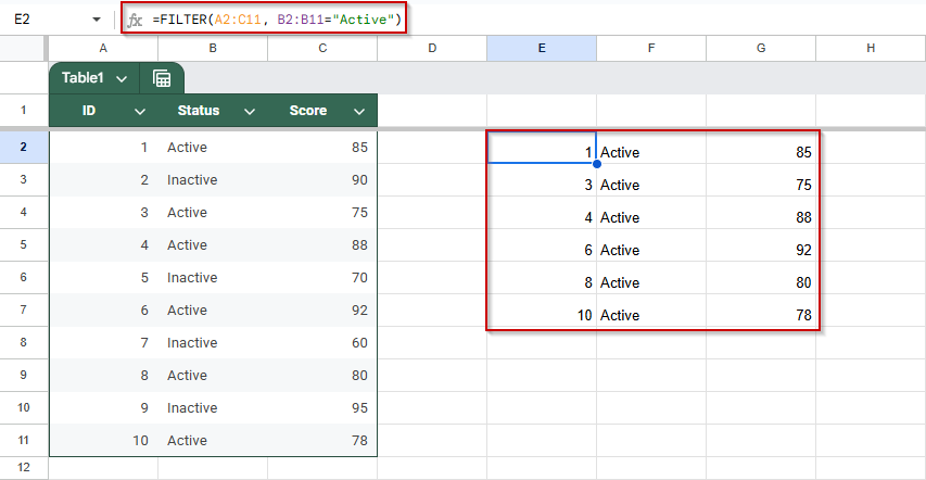
➤ Always match the size of all involved ranges when using multiple conditions.
Frequently Asked Questions
Why is my FILTER formula showing #REF! in Google Sheets?
The #REF! error usually means your filter range and criteria range have mismatched row counts. Ensure all referenced ranges cover the same number of rows.
Why does FILTER return no data even when matches exist?
This happens when the criteria don’t match due to typos, extra spaces, or formatting differences. Use TRIM or CLEAN to sanitize your data and criteria.
Can I use multiple conditions in the FILTER function?
Yes, use * for AND logic and + for OR logic. Group each condition in parentheses to ensure proper evaluation and accurate filtered results.
How do I filter based on partial text matches?
Use REGEXMATCH with FILTER for partial matches. Example:
=FILTER(A2:C11, REGEXMATCH(B2:B11, “Act”)) to return rows with “Active” or similar terms.
Wrapping Up
When the FILTER function in Google Sheets doesn’t work as expected, it’s often due to simple issues like mismatched ranges, incorrect criteria, or hidden formatting problems. By carefully checking your data, using functions like TRIM and CLEAN, and structuring your conditions properly, you can quickly troubleshoot and fix most FILTER errors.