Using a drop-down list in Excel is a powerful way to limit user input, reduce errors, and simplify data entry, especially when working across multiple sheets. When your source data lives on a different worksheet, it allows you to separate raw data from the working area, keeping your main sheet clean and well-organized.
In this article, we’ll walk through several relevant methods to create a drop-down list in Excel using data from another sheet. From basic sheet references to dynamic named ranges, you’ll learn when to use each method and how to apply them step-by-step.
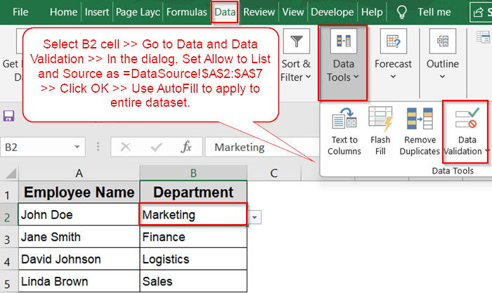
Steps to create a drop-down list from another sheet in Excel:
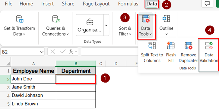
➤ Select B2 cell >> Go to Data and Data Validation under Data Tools.
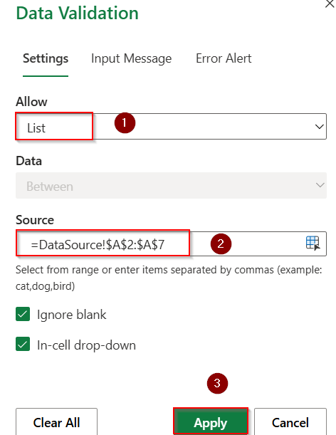
➤ In the dialog, Set Allow to List and Source as =DataSource!$A$2:$A$7
Here, you can replace the formula with your source sheet name and data range.
➤ Click OK to save changes.
➤ Use AutoFill to apply changes to the entire dataset.
Use Direct Sheet Reference for a Fixed List
This method is great for short, fixed lists where you don’t expect the source data to change often. You’ll directly reference the list range on another worksheet using a basic formula inside the Data Validation tool.
Steps:
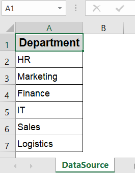
➤ Create a sheet called DataSource where you will list your drop-down data.
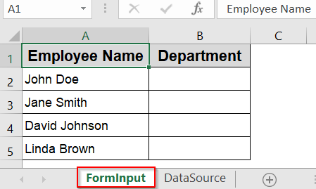
➤ Add a new sheet called FormInput and select cell B2 where the drop-down should appear.
➤ Click on the Data tab and choose Data Validation under Data tools on the ribbon.
➤ In the dialog, set Allow to List.
➤ In the Source box, type:
=DataSource!$A$2:$A$7
You can customise this formula by inserting your source sheet name by starting with an equal sign and inserting your actual data range.
➤ Click Apply to see changes.
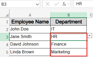
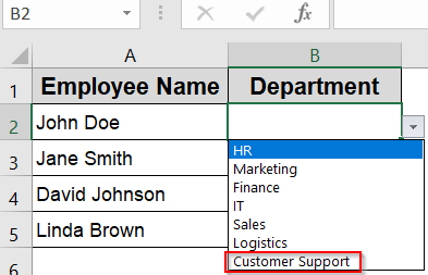
➤ You’ll now see a drop-down in B2 showing all the departments from the DataSource sheet.

➤ Drag down using the AutoFill handle to add a drop-down list for the rest of the cells and select the correct value according to your data.

Create a Named Range from Another Sheet
Named ranges make formulas easier to manage and work across all sheets without typing the full reference every time. This is especially useful if the same list is used in multiple places.
Steps:
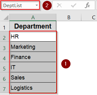
➤ Go to the DataSource sheet and select cells A2:A7.
➤ Click inside the Name Box next to the formula bar, type DeptList, and press Enter.
➤ Now switch to the FormInput sheet and select cell B2.
➤ Click on the Data tab and choose Data Validation under Data tools on the ribbon.

➤ In the dialog, set Allow to List.
➤ In the Source box, type:
=DeptList
➤ Click OK.
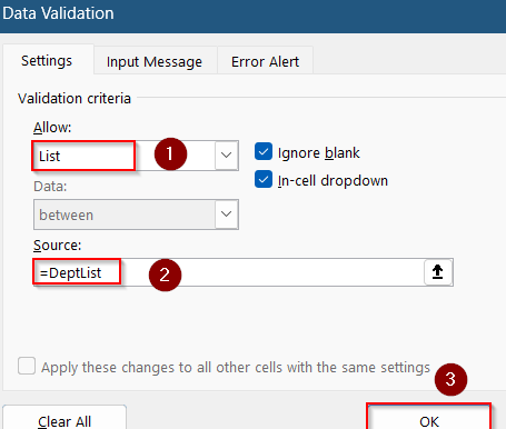
➤ Now the drop-down in cell B2 will pull values directly from the named range DeptList on the other sheet.
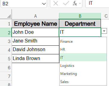
➤ Then you can drag down using the AutoFill handle to add a drop-down list for the rest of the cells and select the correct value according to your data.

Table-Based Drop-Down with Structured References
Converting the source list to a Table lets your drop-down list grow automatically as you add new departments. It’s a smart choice when your list is expected to expand or shrink frequently.
Steps:
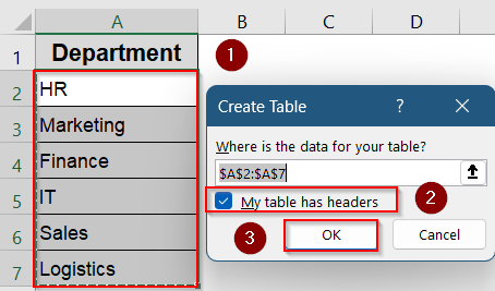
➤ Go to the DataSource sheet and select cells A1:A7, including the header.
➤ Press Ctrl + T to create a Table and make sure “My table has headers” is checked.
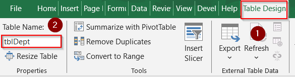
➤ Go to the Table Design tab and rename the table to tblDept.
➤ Now go to the FormInput sheet and select cell B2.
➤ Click on the Data tab and choose Data Validation under Data tools on the ribbon.

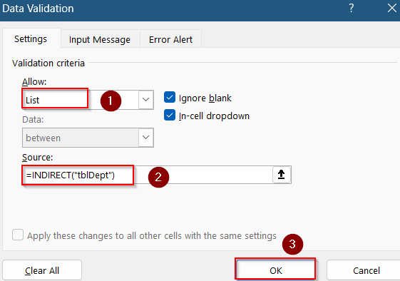
➤ In the dialog, set Allow to List.
➤ Inside Source box, type:
=INDIRECT(“tblDept”)
➤ Click OK.
➤ As the drop-down sign appears, you can now drag down using the AutoFill handle to add a drop-down list for the rest of the cells and select the correct value according to your data.

This method ensures that whenever you add a new department in DataSource sheet such as Customer Support, the drop-down updates automatically.

Build a Dynamic Named Range with OFFSET
If you’re not using a Table but still want automatic expansion of the list, a dynamic named range using the OFFSET function is a flexible solution.
Steps:
➤ On the DataSource sheet, click Formulas >> Name Manager >> New.

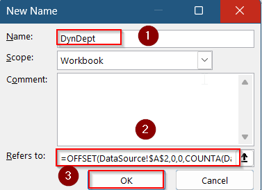
➤ Name your range as DynDept.
➤ In the Refers to box, enter this formula:
=OFFSET(DataSource!$A$2,0,0,COUNTA(DataSource!$A:$A)-1,1)
➤ Click OK to save.
➤ Close the Name Manager dialog box.
➤ Go to the FormInput sheet and select cell B2.
➤ Click on the Data tab and choose Data Validation under Data tools on the ribbon.

➤ In the dialog, set Allow to List.
➤ Inside Source box, type:
=DynDept
➤ Click OK.

➤ As the drop-down sign appears, you can now drag down using the AutoFill handle to add a drop-down list for the rest of the cells and select the correct value according to your data.
Now your drop-down will automatically include any new departments typed below cell A7 in the DataSource sheet such as Customer Support.
Combine Unique with Spill Range (Excel 365 Only)
Excel 365 users can take advantage of dynamic arrays to create a real-time drop-down that shows only unique, sorted values. This works well if your source list might contain duplicates or needs sorting.
Steps:
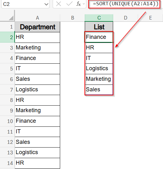
➤ Go to the DataSource sheet and select an empty column, say C2.
➤ Enter this formula to extract and sort unique values:
=SORT(UNIQUE(A2:A14))
➤ Press Enter and Excel will spill the results automatically.
➤ Now switch to the FormInput sheet and click cell B2.
➤ Click on the Data tab and choose Data Validation under Data tools on the ribbon.

➤ In the dialog, set Allow to List.
➤ Inside Source box, type:
=DataSource!$C$2#
➤ Click Apply to save changes.
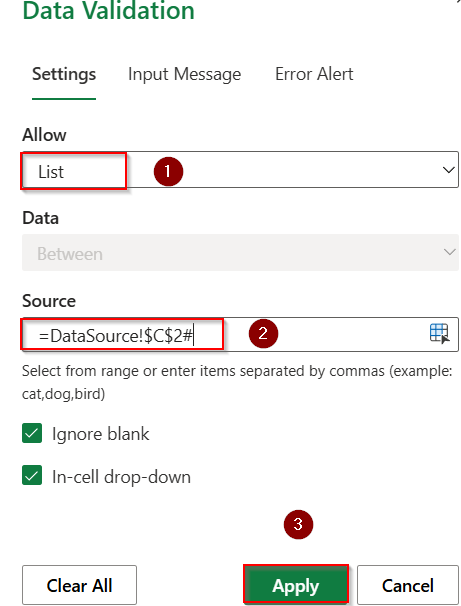
➤ The # sign tells Excel to include the entire spill range. The drop-down in B2 now reflects only unique, sorted department names.

➤ You can now drag down using the AutoFill handle to add a drop-down list for the rest of the cells and select the correct value according to your data.

Create a Drop-Down List from Another Workbook
You can even create a drop-down list using data from a completely different workbook. This is useful when multiple files need to share the same validation rules. But, keep in mind that both workbooks must be open.
Steps:
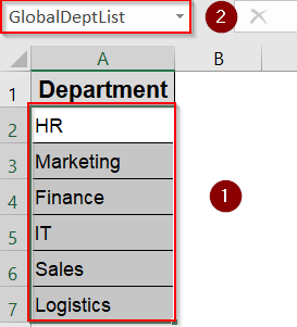
➤ In your source workbook, go to DataSource and select A2:A7.
➤ Define this as a named range (e.g., GlobalDeptList) via the Name Box.
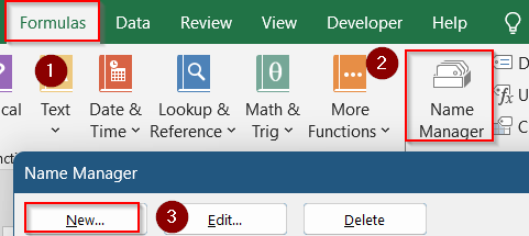
➤ Now open your target workbook and go to Formulas >> Name Manager >> New.
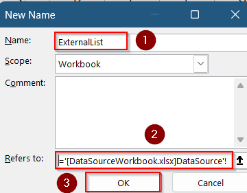
➤ Name it ExternalList.
➤ In the Refers to box, type something like:
='[DataSourceWorkbook.xlsx]DataSource’!GlobalDeptList
➤ Click OK.
➤ Close the Name Manager dialog box.

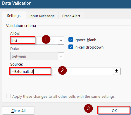
➤ Click on the Data tab and choose Data Validation under Data tools on the ribbon.

➤ In the dialog, set Allow to List.
➤ For Source, enter:
=ExternalList
➤ Click OK.
➤ You can drag down using the AutoFill handle to add a drop-down list for the rest of the cells and select the correct value according to your data.

You’ll now have a drop-down in one workbook that references a named list from another but make sure both workbooks remain open when using it.
Frequently Asked Questions
Can I protect drop-down list items from being changed by users?
Yes. You can protect the source sheet with a password and hide it to prevent edits. Also, enable the Error Alert in Data Validation to block users from typing invalid entries.
How do I remove a drop-down list from a cell?
Select the cell, go to Data and click on Data Validation, then click Clear All. This removes the drop-down, but any existing value will remain unless you delete it manually.
What happens if the list source contains blank cells?
Blank cells will appear as empty options in the drop-down. To avoid this, use dynamic named ranges, Excel Tables, or ensure your source range contains only filled values.
Can I use a drop-down list from another workbook?
Yes, but both workbooks must be open. Define a named range in the source file, then reference it in the destination workbook. It won’t work if the source file is closed.
Wrapping Up
In this tutorial, we learned multiple practical methods to create an Excel drop-down list using data from another sheet. These methods range from simple direct references to advanced dynamic named ranges and UNIQUE spill formulas that allow you to build smarter, scalable, and more maintainable dropdowns based on your data source. Feel free to download the practice file and share your feedback.