If you manage multiple spreadsheets in Google Sheets, the IMPORTRANGE function lets you pull live data from one sheet into another. Whether you’re consolidating reports, building dashboards, or separating input and output data, this function keeps everything connected and up to date automatically.
In this article, you’ll learn how to use the IMPORTRANGE formula step-by-step, along with practical use cases, sample datasets, and pro tips for avoiding common errors.
Steps to import a basic range from a source sheet:
➤ Open your destination Google Sheet (e.g., “Team Dashboard“) and select cell A1.
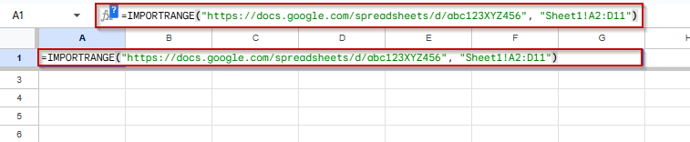
➤ Enter the formula:
=IMPORTRANGE(“https://docs.google.com/spreadsheets/d/abc123XYZ456”, “Sheet1!A2:D11”)
➤ Replace the URL with the link to your actual source spreadsheet (e.g., “Sales Report Q1“).
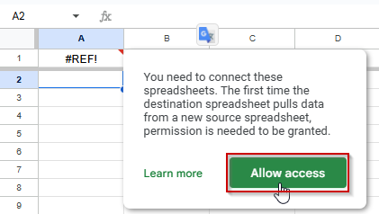
➤ When prompted, click Allow Access to connect the two spreadsheets.
➤ Your selected range (A2:D11) will appear instantly in the destination sheet.
➤ Any updates in the source sheet, like changes in sales data, will sync automatically in real time.

Import a Simple Range from Another Google Sheet
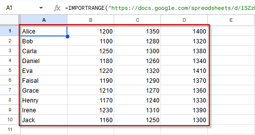
If you’re managing data across multiple spreadsheets, the IMPORTRANGE function is the simplest way to pull live data from one Google Sheet into another. Whether you’re combining monthly reports or referencing a central data source, this method keeps your files connected and automatically synced. In this example, we’ll import a 10-row dataset from a source sheet that tracks employee sales data.
This is the source sheet (Sales Report Q1) that we will use to demonstrate the methods:
 In addition, we will use a blank destination sheet (Team Dashboard) to import the ranges from the source sheet.
Steps:
➤ Open your destination Google Sheet and click on cell A1
➤ Type the following formula (replacing the URL with your actual source sheet’s link):
=IMPORTRANGE(“https://docs.google.com/spreadsheets/d/abc123XYZ456”, “Sheet1!A2:D11”)
➤ If it’s your first time importing from this source, click Allow Access when prompted.
The employee sales data will appear in your destination sheet automatically.

➤ Any updates to the source spreadsheet (e.g., new March figures) will reflect live in your imported table.
Using IMPORTRANGE function to Import Data from a Named Range in Another Google Sheet
Using a named range with IMPORTRANGE function is ideal when you’re working with structured data like reports or tables that may move or expand. Instead of specifying a static range like “Sheet1!A2:D11“, you can assign a name to that range (e.g., “Sales2024“) in the source sheet. This makes your formula easier to read and maintain.
Steps:
➤ Open your source Google Sheet.
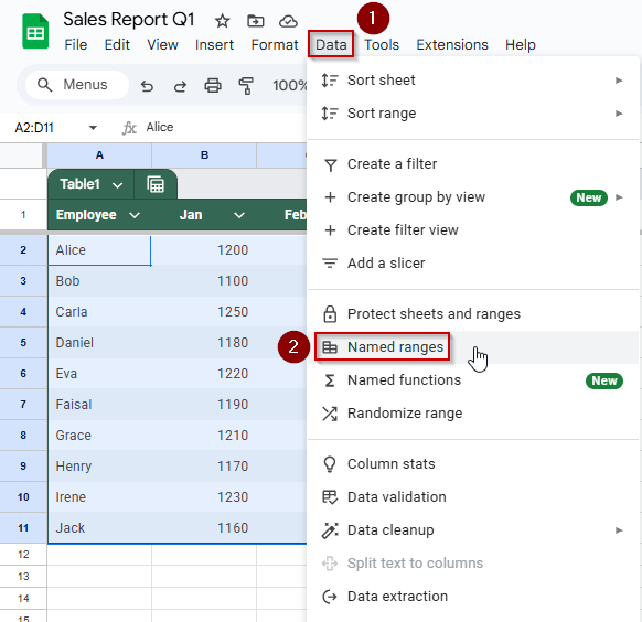
➤ Highlight the range you want to import, for example, A2:D11.
➤ Go to Data >> Named ranges.
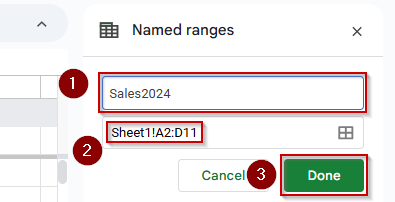
➤ In the sidebar that appears, enter a name (e.g., Sales2024) and click Done.
➤ In the destination sheet, select the cell where you want the imported data to begin (e.g., A1).
➤ Type the following formula (Replace the URL with the URL with your source sheet):
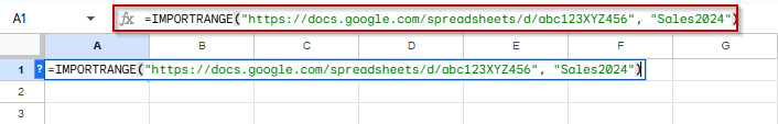
=IMPORTRANGE(“https://docs.google.com/spreadsheets/d/abc123XYZ456”, “Sales2024”)
➤ On first use, you’ll be prompted with Allow access, click it to link the spreadsheets.
Your named range will now populate in the destination sheet, and it will update automatically as the source data changes.
Combining IMPORTRANGE and FILTER Functions to Import Only Matching Rows in Google Sheets
If you only need to bring in certain rows, like all records for a specific employee, you can combine the IMPORTRANGE and FILTER functions. This method is perfect for focused reports or dashboards where importing everything would clutter your sheet.
Steps:
➤ Click on cell A1 in your destination sheet (where you want the filtered data to appear).
➤ Enter the following formula:
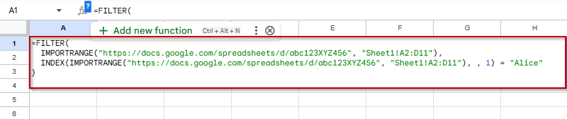
=FILTER(
IMPORTRANGE(“https://docs.google.com/spreadsheets/d/abc123XYZ456”, “Sheet1!A2:D11”),
INDEX(IMPORTRANGE(“https://docs.google.com/spreadsheets/d/abc123XYZ456”, “Sheet1!A2:D11”), , 1) = “Alice”
)
➤ The first time you use IMPORTRANGE, click Allow Access when prompted.
➤ This formula pulls the full dataset, but FILTER only shows rows where column A (Employee) is Alice.
➤ You can also replace “Alice” with another candidate or value for dynamic filtering.
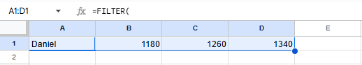
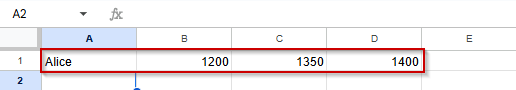
Only the relevant data now appears, reducing clutter and making analysis easier.
Frequently Asked Questions
Why Does IMPORTRANGE show a #REF! Error?
The #REF! error usually appears when access hasn’t been granted to the source sheet. Click “Allow access” to authorize the connection between sheets.
Can I use IMPORTRANGE across different Google accounts?
Yes, but the destination account must be granted viewing or editing access to the source sheet. Without permissions, IMPORTRANGE won’t retrieve any data.
Does IMPORTRANGE update automatically when the source data changes?
Yes, IMPORTRANGE is dynamic. Any changes in the source sheet reflect automatically in the destination sheet without needing to refresh manually.
Can I use IMPORTRANGE with QUERY or FILTER?
Absolutely. IMPORTRANGE can be wrapped with QUERY or FILTER to import only specific rows or columns based on conditions, allowing more control over the imported data.
Wrapping Up
Using IMPORTRANGE in Google Sheets is a powerful way to link data across files, whether you’re combining reports, managing shared inputs, or building dynamic dashboards. From simple cell ranges to named ranges and filtered imports, these methods help you centralize data without manual copy-pasting. Choose the approach that fits your workflow and enjoy smooth, real-time updates between sheets.