When we are working with data tables it’s a common thing to make the first row as a header. This is needed when you want to clearly identify the content of each column and additionally to enable some features like data filtering, sorting and analysis. Typically, this need arises when we import data from external sources, copying data. If Excel does not automatically recognize your first row as the header we definitely need this.
To make first row as header in Excel, follow these simple steps:
➤ Select the data range including the first row.
➤ Convert the data into an Excel Table using Ctrl + T or Home > Format as Table.
➤ Make sure the checkbox “My table has headers” is selected and click OK.
In this article, we’ll show you three methods to make the first row as the header in Excel. You’ll learn how to do this using Excel Tables, Power Query and Freeze Panes.
Applying Freeze Panes Feature To Make First Row as Header
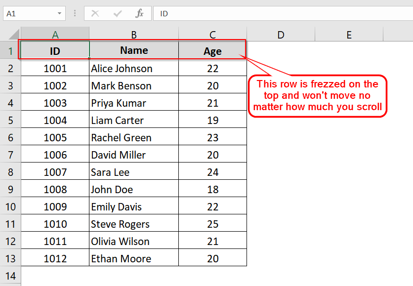
This Freeze Panes method can keep the first row of the Excel sheet visible as you scroll down. It is useful when you’re working with large datasets like employee records, attendance sheets, or product lists and where column headers are needed to be on the top for reference during navigation.
Steps:
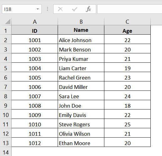
➤ Open your Excel file that contains a data table. Your dataset may span from A1 to C50, but the first row should contain text that can work as headers. For example: “Employee ID”, “Name”, “Days Present”.
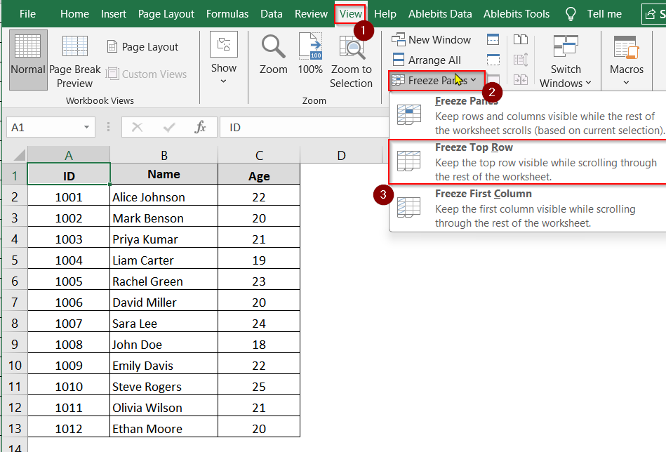
➤ Click on the “View” tab in the Ribbon at the top of Excel. In the “Window” group, click the “Freeze Panes” dropdown button. From the dropdown, click “Freeze Top Row.” You will not see any visual changes, but the top row is now locked.
➤ Now scroll down your sheet. You’ll notice the first row stays in place, no matter how much you scroll.
Notes:
➧ This method only locks the topmost visible row. If your header is not in Row 1, use the general Freeze Panes
➧ To unfreeze, go to the same menu and click “Unfreeze Panes.”
Implementing Data to Excel Table Convert Method To Make First Row Header
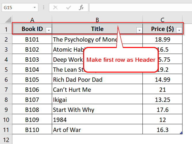
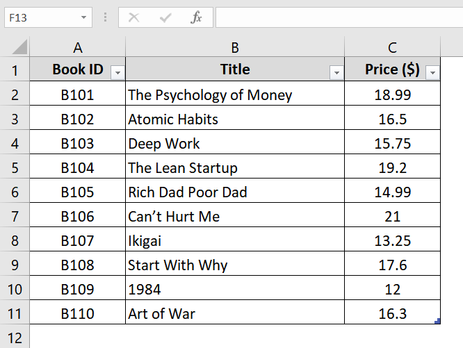
Converting your Data To Excel Table method can transform your dataset into an Excel Table. In the excel table the first row is automatically treated as the header. It also activates some built in features like sorting, filtering, formatting, and easy formula referencing. You should use it when working with inventory, sales logs, student lists, and other structured data.
Steps:
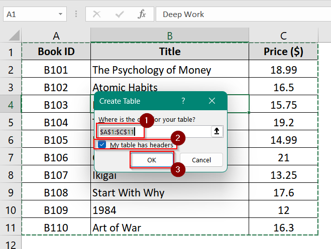
➤ Select A1 to C11 for a table with Book ID, Title, and Price.
➤ Click the “Home” tab on the Ribbon at the top of Excel.
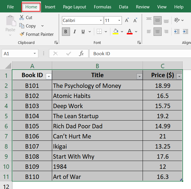
➤ In the Styles group, click the “Format as Table” button. A dropdown will appear showing various table styles.
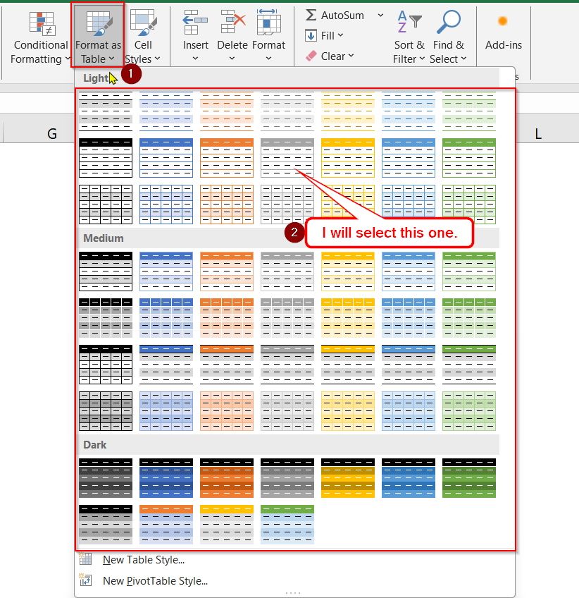
➤ Click any table style you prefer. A dialog box titled “Create Table” will pop up.
➤ In the “Create Table” dialog box:
- Make sure the checkbox “My table has headers” is selected.
- Your selected range (like $A$1:$C$11) should appear in the input box.
➤ Then click OK.
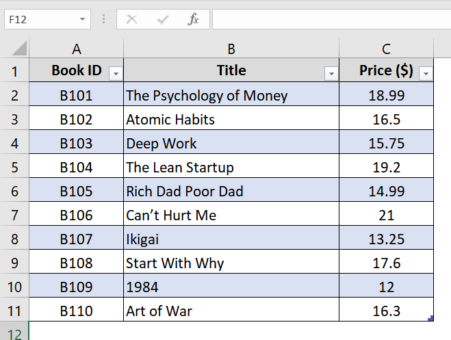
➤ Your data is now converted into an Excel Table where the first row is a header row.
Notes:
➧ If you forget to check “My table has headers,” Excel will treat the first row as data. You can fix this by Going to the “Table Design” tab > Check “Header Row.”
➧ You can use the shortcut Ctrl + T for faster table creation.
Using Power Query Editor to Make First Row Header in Excel
This method uses Power Query. It is a powerful Excel tool that can also convert the first row of a dataset into header columns. It is ideal when you are importing raw data from external sources (CSV, web, or copy-paste) and where the headers aren’t properly recognized.
Steps:
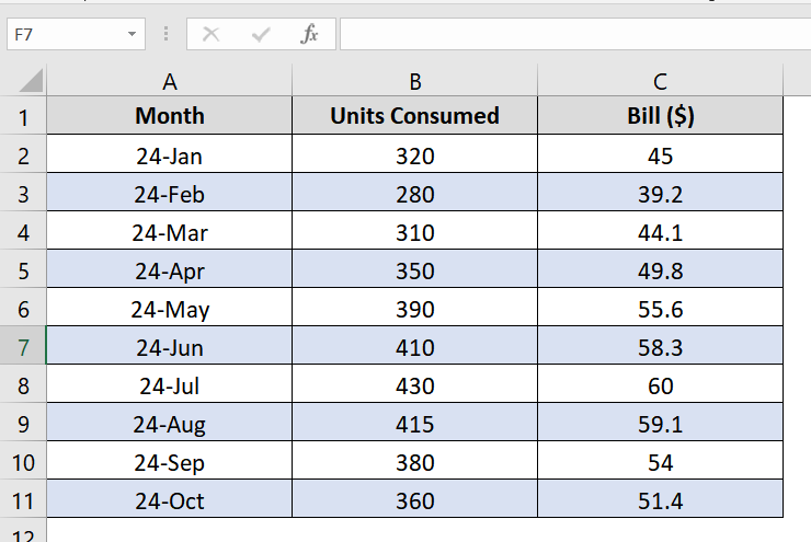
➤ Select the range A1:C11 which includes the header row and 10 months of data.
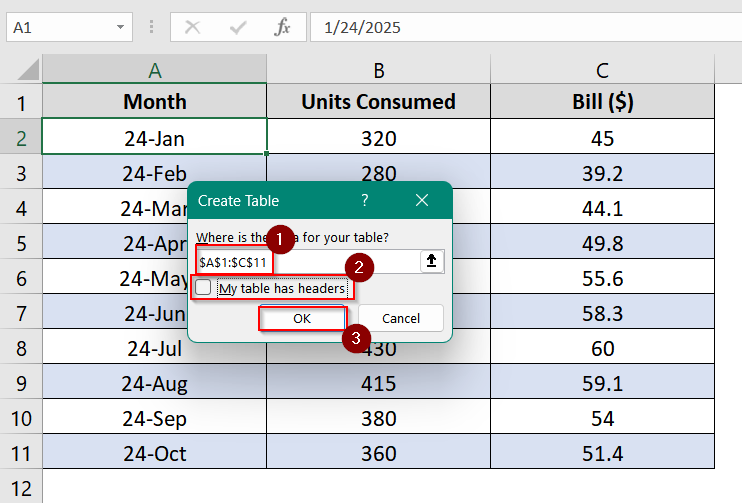
➤ Navigate to the Data tab in the Excel ribbon.
➤Click on “From Table/Range” under the Get & Transform Data group.
➤ A dialog box appears titled Create Table. Ensure the checkbox for “My table has headers” is unchecked, since we’ll set headers manually in Power Query.
➤ Click OK.
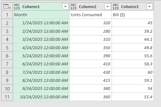
➤ Your data now appears in the Power Query Editor where the first row (e.g., “Month”, “Units Consumed”, “Bill ($)”) is still shown as regular data.
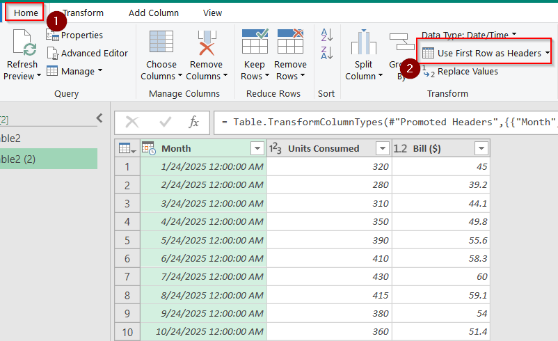
➤ Go to the Home tab in Power Query Editor.
➤ Click “Use First Row as Headers” under the Transform group.
➤ Click the Close & Load button on the Home tab.
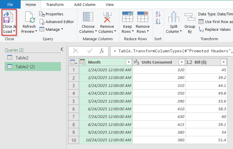
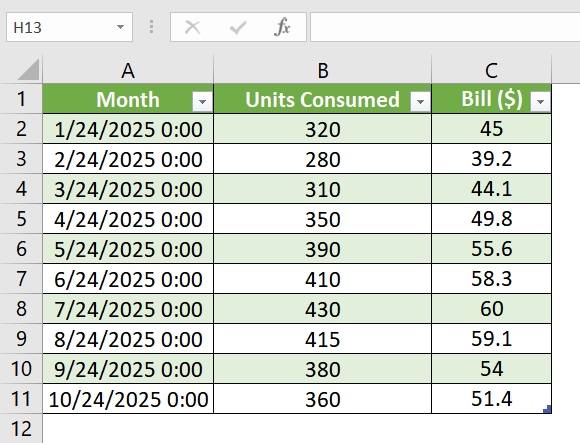
➤ Your cleaned data will load back into a new Excel worksheet with proper headers.
Notes:
➧ Power Query doesn’t change your original sheet; it creates a new output sheet.
➧ You can edit or refresh the query later by going to Queries & Connections on the right panel.
Frequently Asked Questions
Why doesn’t Excel recognize my first row as a header?
Sometimes Excel treats the first row as data if the dataset is imported from other sources or pasted without formatting. Here, you need to define the first row as headers..
Can I make the first row stay visible while scrolling?
Yes!. Use the Freeze Panes > Freeze Top Row option under the View tab to keep the first row visible when you scroll through large datasets.
How do I repeat the header row on every printed page?
Use the Page Layout > Print Titles feature, then set the first row to repeat at the top of each printed page..
What if my headers are not unique or need editing?
Use Power Query Editor to load the data, make the first row as headers, and edit or clean the headers before loading back to Excel.
Concluding Words
I have showeld 3 easy methods on how to make the first row a header in Excel. As you know, it is an essential thing to learn to clear data presentation and spreadsheet management. You can use any of these 3 methods which suits you- converting data to Excel tables, using Power Query, freezing panes and it will automatically make your first row as heading.