You can split your Excel sheet into multiple worksheets depending on a specific data value. It can keep your large and related information organized and simplify your workflow in Excel.
➤ Worksheet splitting means separating data into multiple sheets based on one specific value.
➤ PivotTable: Insert >> PivotTable >> Add filter >> Analyze tab >> Show Report Filter Pages >> OK.
➤ VBA: Developer tab >> Visual Basic >> Insert >> Module >> Writer script >> Run via Macros.
➤ Manual: Manually copy & paste data or use Power Query.
In this article, we will learn three methods to split one Excel sheet into multiple worksheets — one using PivotTable, the other with VBA Script, and last of all, manually.
What Does It Mean to Split an Excel Sheet into Multiple Worksheets?
Splitting a worksheet in Excel into multiple worksheets means dividing a large data sheet into separate sheets based on specific criteria of the given data. We can do so by both column value and row value. It makes it easier to manage or analyze data grouped in categories.
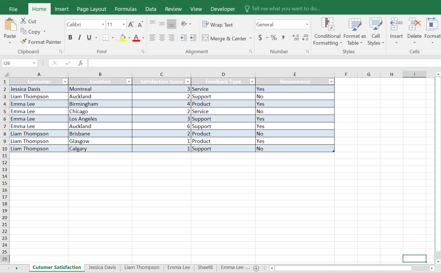
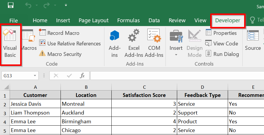
In the following dataset, we have feedback data from multiple customers. First, we are going to split the sheet based on the Customer column, each one will get their own worksheet.
Split the Excel Sheet into Multiple Worksheets Using PivotTable
PivotTable can quickly divide your data into separate sheets using a report filter. Follow the steps below.
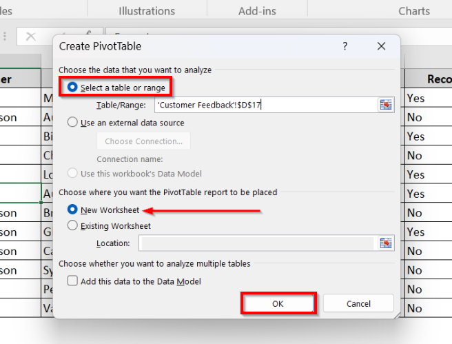
➤ Head over to Insert >> Then PivotTable.
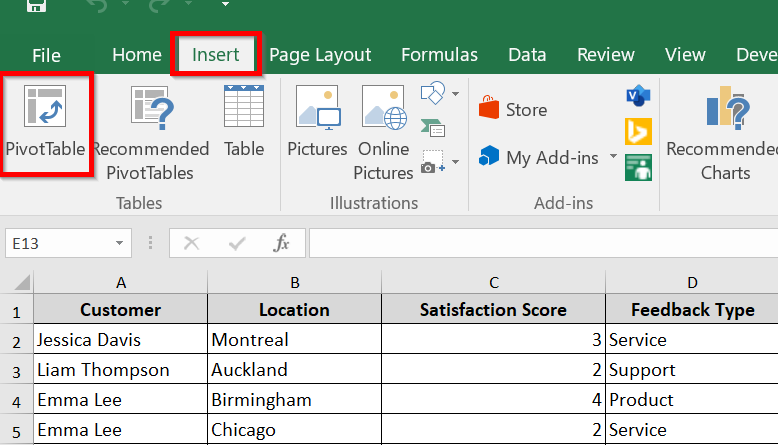
➤ Select a table range. We are okay with the table range. We are just going to make a new sheet. Click on OK.
Note:
Click inside your data first. Then go to Insert >> PivotTable, and Excel should auto-select the correct range.
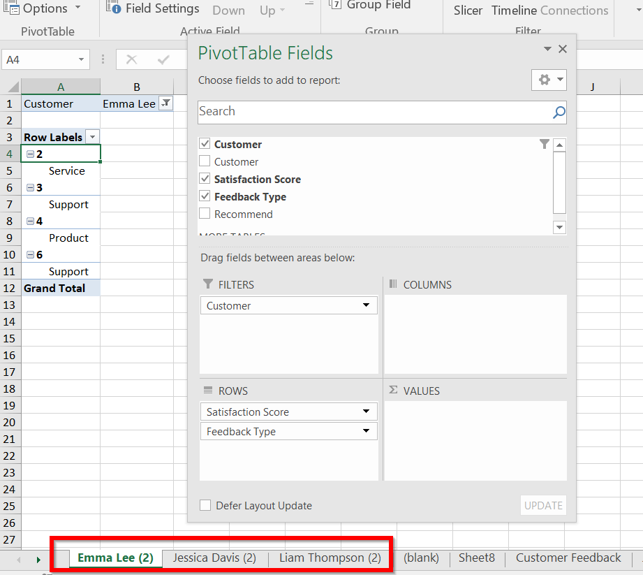
➤ PivotTable Fields will appear. As we are working with the Customer column here, it is important to select and put the Customer as our filter.
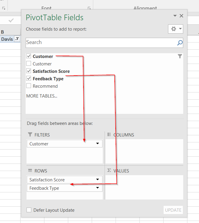
➤ We can extract the relevant data to COLUMN, ROWS, or VALUES as you prefer. Here we’ve selected Satisfaction Score and Feedback Types as rows. This is what it looks like.
➤ Now move to the Analyze tab >> Head to the Options section.
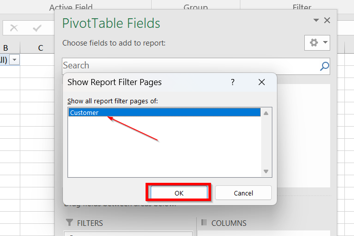
➤ Click on the drop-down menu and select Show Report Filter Pages.
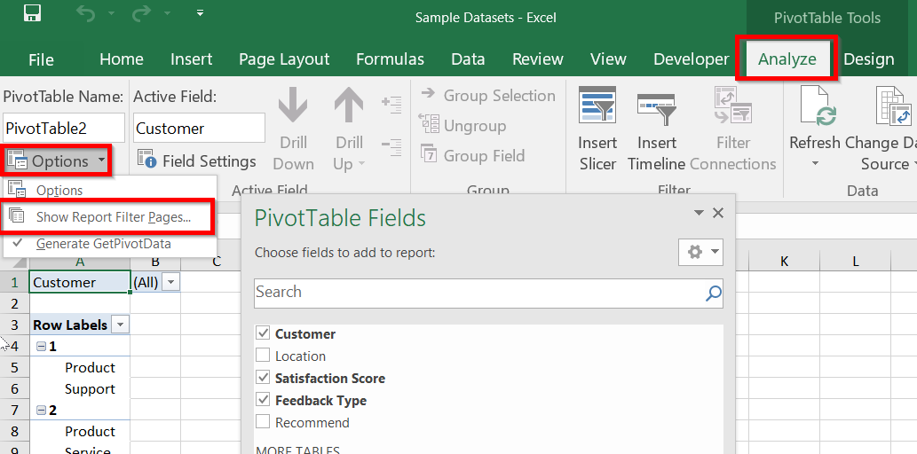
➤ In the pop-up, we want to select Customer as our filter. Click Ok.
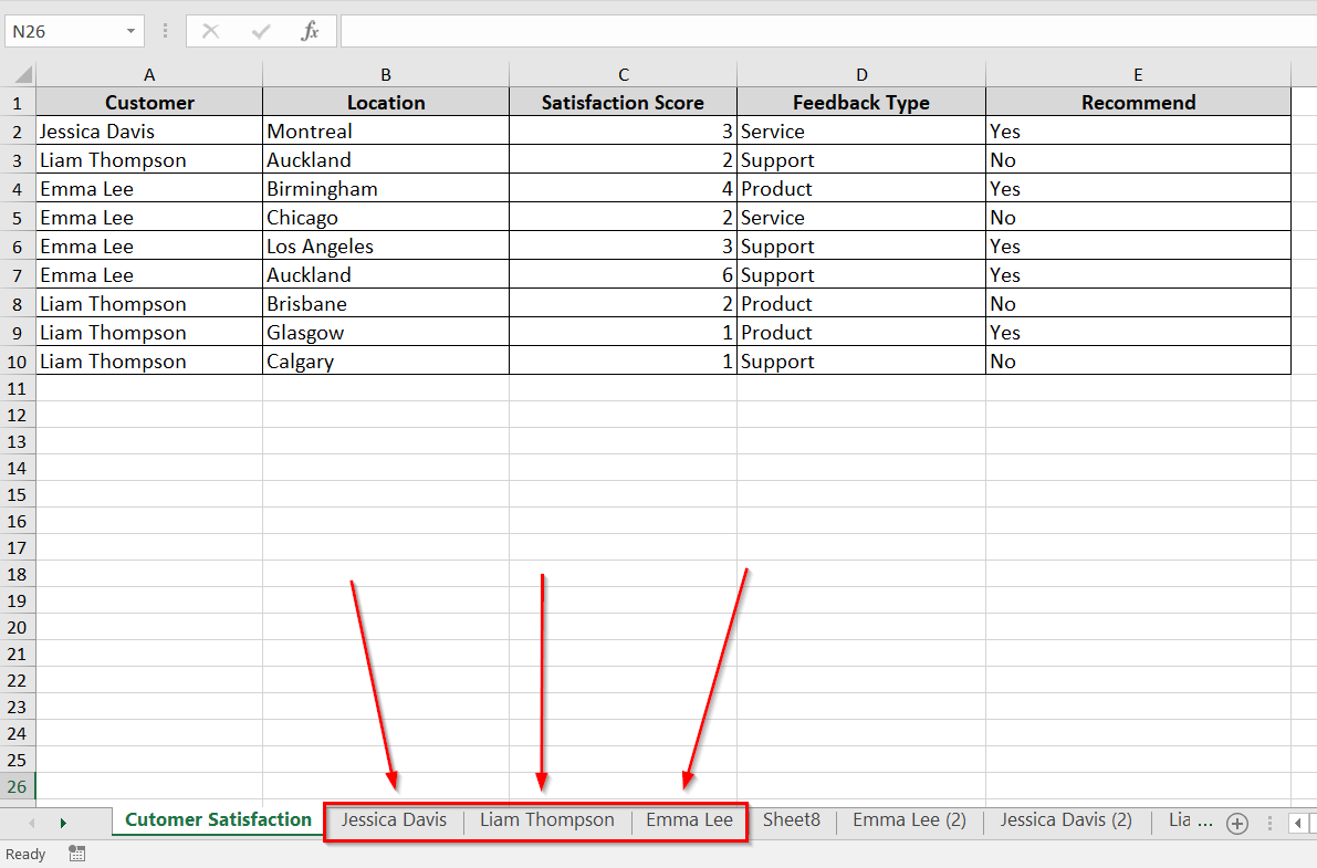
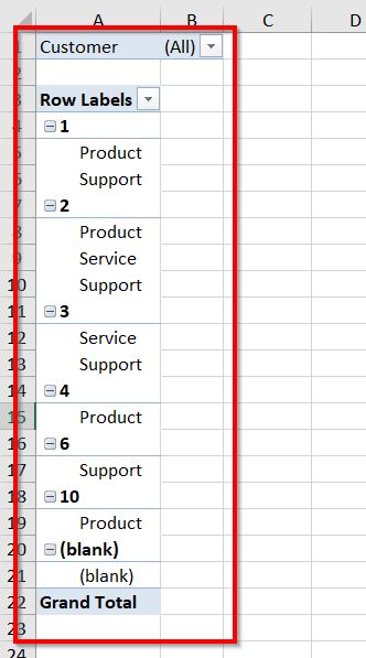
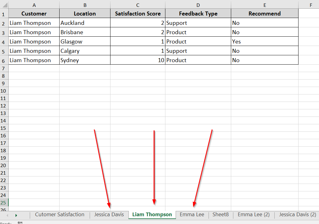
Now you will notice that it has automatically generated three different sheets for each of our three customers.
The best part is that it is fully customizable. Let’s say you want to see by satisfaction score or feedback type, just drag the option as the filter and do the exact same action.
Split an Excel Sheet Based on Column using VBA Script
We have the same table as before, and we’ll split the data by Customer once again using VBA code.
➤ Go to the Developer tab >> Visual Basic
Note:
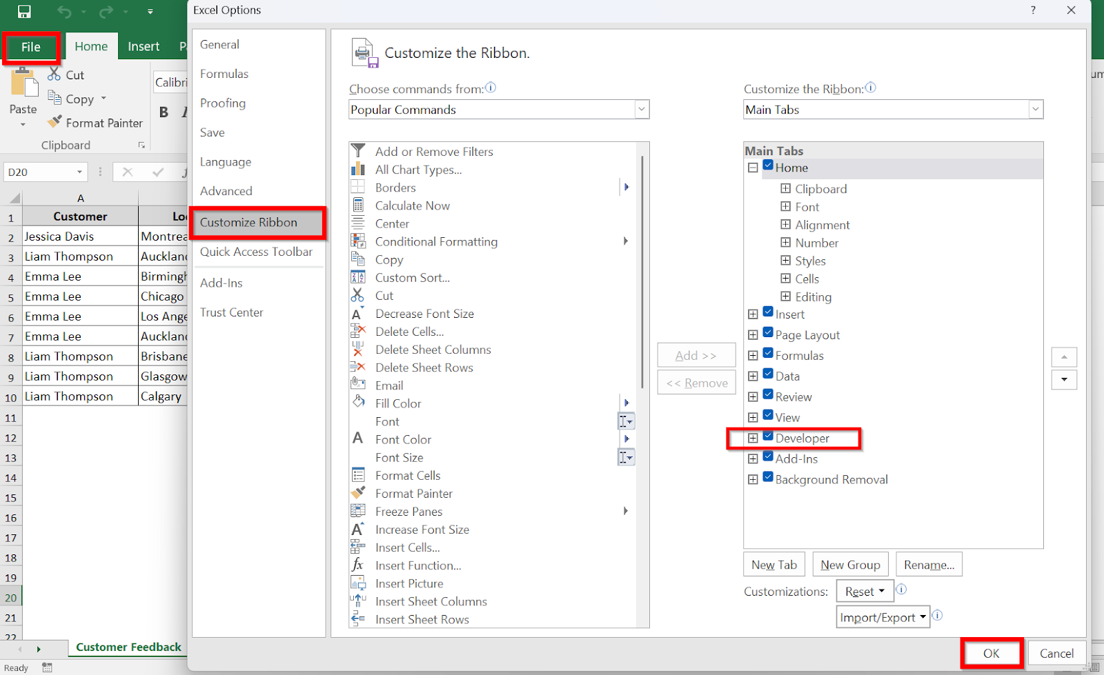
If you don’t see the Developer tab, it’s probably deactivated. Go File >> Options >> Customize Ribbon and tick the Developer tab.
➤ Select Insert from the menu bar >> Click on Module.
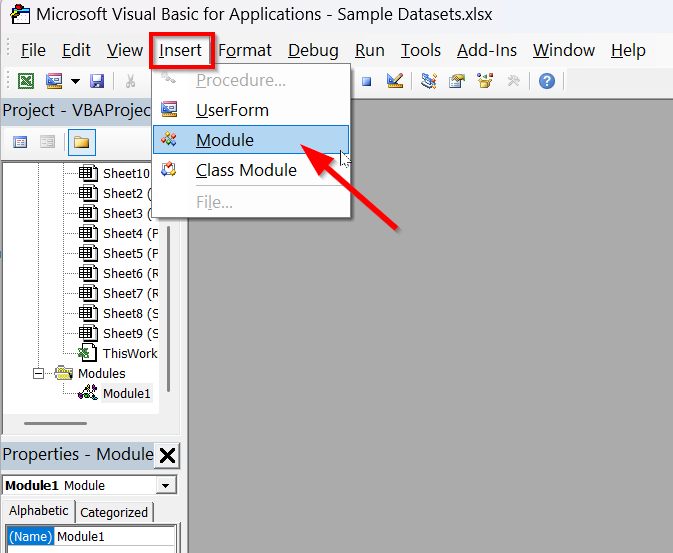
➤ In the module, you will need to write the following VBA code to split the sheets.
You can just copy the code and paste it into the module.
Sub SplitDataBySelectedColumn()
    Dim ws As Worksheet
    Dim wsNew As Worksheet
    Dim rng As Range
    Dim lastRow As Long
    Dim lastCol As Long
    Dim uniqueValues As Collection
    Dim cell As Range
    Dim value As Variant
    Dim colToFilter As Long
    Dim columnHeader As String
    Dim headerFound As Boolean
    Dim i As Long
    Dim sanitizedValue As String
    ' Use the active worksheet
    Set ws = ActiveSheet
    lastRow = ws.Cells(ws.Rows.Count, 1).End(xlUp).Row
    lastCol = ws.Cells(1, ws.Columns.Count).End(xlToLeft).Column
    Set rng = ws.Range(ws.Cells(1, 1), ws.Cells(lastRow, lastCol))
    ' Prompt the user to select the column header
    columnHeader = InputBox("Enter the column header to split the data by (case-insensitive):")
    If columnHeader = "" Then
        MsgBox "No column header entered. Exiting.", vbExclamation
        Exit Sub
    End If
    ' Find the column based on header value (case-insensitive)
    headerFound = False
    For colToFilter = 1 To lastCol
        If LCase(ws.Cells(1, colToFilter).Value) = LCase(columnHeader) Then
            headerFound = True
            Exit For
        End If
    Next colToFilter
    If Not headerFound Then
        MsgBox "Column header not found. Please try again.", vbExclamation
        Exit Sub
    End If
    ' Create a collection of unique values in the selected column
    Set uniqueValues = New Collection
    On Error Resume Next
    For Each cell In ws.Range(ws.Cells(2, colToFilter), ws.Cells(lastRow, colToFilter))
        uniqueValues.Add cell.Value, CStr(cell.Value)
    Next cell
    On Error GoTo 0
    ' Loop through unique values and create a new worksheet for each
    For Each value In uniqueValues
        ' Sanitize value for worksheet name
        sanitizedValue = Replace(CStr(value), "/", "_")
        sanitizedValue = Replace(sanitizedValue, "\", "_")
        sanitizedValue = Replace(sanitizedValue, "*", "_")
        sanitizedValue = Replace(sanitizedValue, "[", "_")
        sanitizedValue = Replace(sanitizedValue, "]", "_")
        sanitizedValue = Left(sanitizedValue, 31) ' Truncate to 31 characters if needed
        ' Check if the sheet name is valid and unique
        On Error Resume Next
        Set wsNew = ThisWorkbook.Sheets(sanitizedValue)
        On Error GoTo 0
        If wsNew Is Nothing Then
            ' Add a new worksheet and name it after the sanitized unique value
            Set wsNew = ThisWorkbook.Sheets.Add(After:=ThisWorkbook.Sheets(ThisWorkbook.Sheets.Count))
            wsNew.Name = sanitizedValue
        Else
            Set wsNew = Nothing
            GoTo NextValue
        End If
        ' Copy the headers
        ws.Rows(1).Copy Destination:=wsNew.Rows(1)
        ' Copy matching rows directly without filtering
        i = 2 ' Start pasting from row 2 in the new sheet
        For Each cell In ws.Range(ws.Cells(2, colToFilter), ws.Cells(lastRow, colToFilter))
            If cell.Value = value Then
            cell.EntireRow.Copy wsNew.Rows(i)
            i = i + 1
            End If
        Next cell
NextValue:
        Set wsNew = Nothing
    Next value
End Sub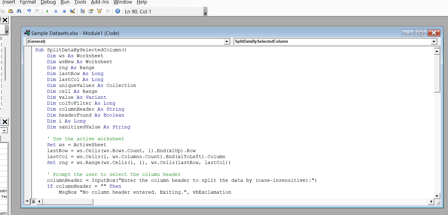
➤ Close the VBA editor now and go back to your worksheet.
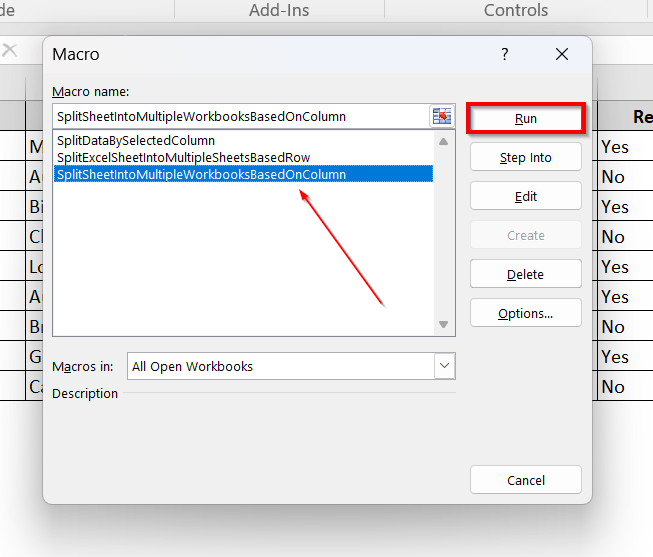
➤ Next, select Macros. Select the specific Macro and run it.
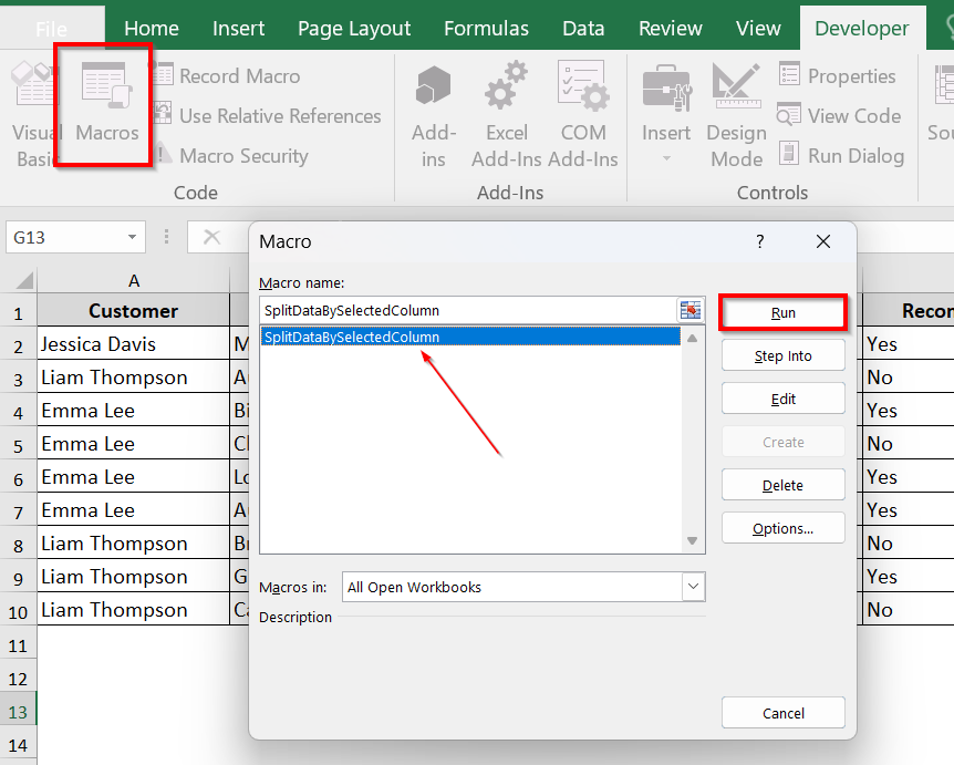
It will automatically create three new worksheets. Have a look at the result in the hands-on example below.
Split Excel Sheet Into Multiple Worksheets Based On Rows Using VBA Script
As an alternative, now we will split sheets based on rows. For this, in the same worksheet, we have reduced the number of rows to 10.
➤ Go to Developer tab >> Visual Basic >> Insert >> Click on Module.
➤ In the module, write the script and close it.
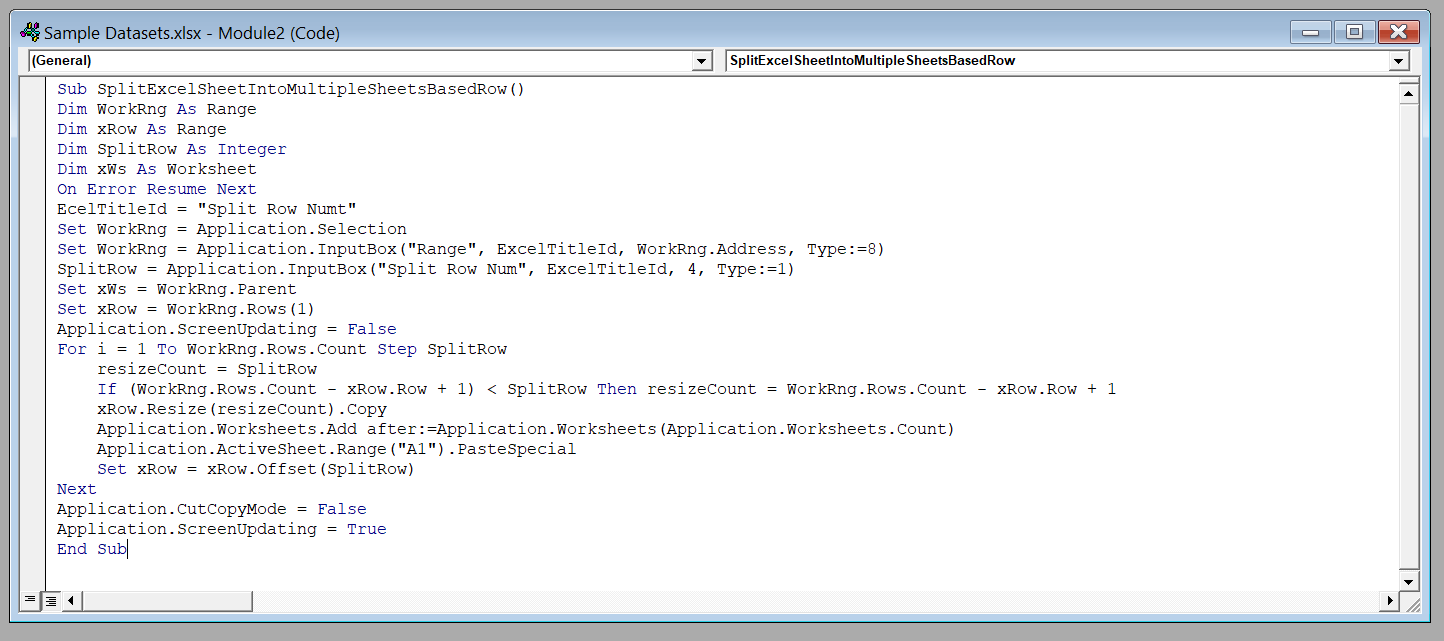
We have added the following script.
Sub SplitExcelSheetIntoMultipleSheetsBasedRow()
Dim WorkRng As Range
Dim xRow As Range
Dim SplitRow As Integer
Dim xWs As Worksheet
On Error Resume Next
EcelTitleId = "Split Row Numt"
Set WorkRng = Application.Selection
Set WorkRng = Application.InputBox("Range", ExcelTitleId, WorkRng.Address, Type:=8)
SplitRow = Application.InputBox("Split Row Num", ExcelTitleId, 4, Type:=1)
Set xWs = WorkRng.Parent
Set xRow = WorkRng.Rows(1)
Application.ScreenUpdating = False
For i = 1 To WorkRng.Rows.Count Step SplitRow
resizeCount = SplitRow
If (WorkRng.Rows.Count - xRow.Row + 1) < SplitRow Then resizeCount = WorkRng.Rows.Count - xRow.Row + 1
xRow.Resize(resizeCount).Copy
Application.Worksheets.Add after:=Application.Worksheets(Application.Worksheets.Count)
Application.ActiveSheet.Range("A1").PasteSpecial
Set xRow = xRow.Offset(SplitRow)
Next
Application.CutCopyMode = False
Application.ScreenUpdating = True
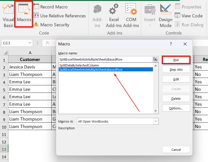
End Sub➤ Then again, we will return to Macros. Select the specific macro and run it.
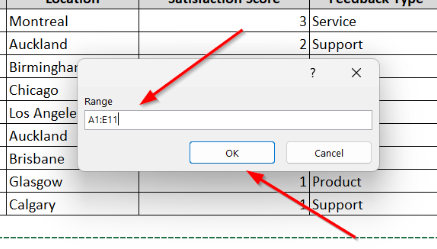
➤ You will be asked to select a range. For our sheet, we have selected A1:E11 [Column A to E, Row 1 to Row 11].
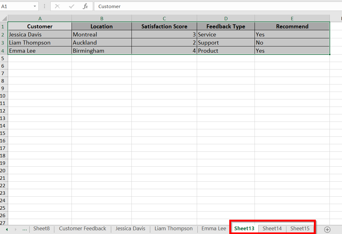
➤ Specify the Row number to split by. We have selected four, and Macro has returned to three new worksheets.
VBA Script To Split an Excel Sheet into Multiple Files
Now we are going to split the Excel sheet into multiple files with the help of a VBA script.
➤ Go to Developer tab >> Visual Basic >>
➤ Move to Insert >> Click on Module.
➤ In the module, write the VBA script.
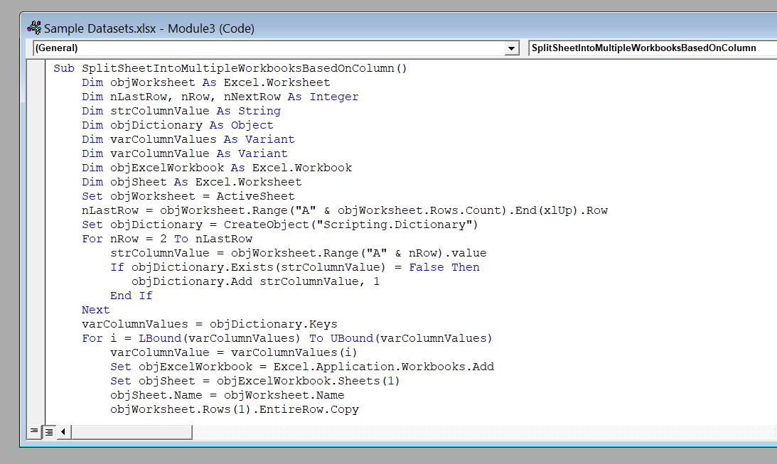
We have used this script. You can just copy and paste it.
Sub SplitSheetIntoMultipleWorkbooksBasedOnColumn()
Dim objWorksheet As Excel.Worksheet
Dim nLastRow, nRow, nNextRow As Integer
Dim strColumnValue As String
Dim objDictionary As Object
Dim varColumnValues As Variant
Dim varColumnValue As Variant
Dim objExcelWorkbook As Excel.Workbook
Dim objSheet As Excel.Worksheet
Set objWorksheet = ActiveSheet
nLastRow = objWorksheet.Range("A" & objWorksheet.Rows.Count).End(xlUp).Row
Set objDictionary = CreateObject("Scripting.Dictionary")
For nRow = 2 To nLastRow
strColumnValue = objWorksheet.Range("A" & nRow).Value
If objDictionary.Exists(strColumnValue) = False Then
objDictionary.Add strColumnValue, 1
End If
Next
varColumnValues = objDictionary.Keys
For i = LBound(varColumnValues) To UBound(varColumnValues)
varColumnValue = varColumnValues(i)
Set objExcelWorkbook = Excel.Application.Workbooks.Add
Set objSheet = objExcelWorkbook.Sheets(1)
objSheet.Name = objWorksheet.Name
objWorksheet.Rows(1).EntireRow.Copy
objSheet.Activate
objSheet.Range("A1").Select
objSheet.Paste
For nRow = 2 To nLastRow
If CStr(objWorksheet.Range("A" & nRow).Value) = CStr(varColumnValue) Then
objWorksheet.Rows(nRow).EntireRow.Copy
nNextRow = objSheet.Range("A" & objWorksheet.Rows.Count).End(xlUp).Row + 1
objSheet.Range("A" & nNextRow).Select
objSheet.Paste
objSheet.Columns("A:F").AutoFit
End If
Next
Next
End Sub
➤ Return to Macros. Select the specific macro and run it.
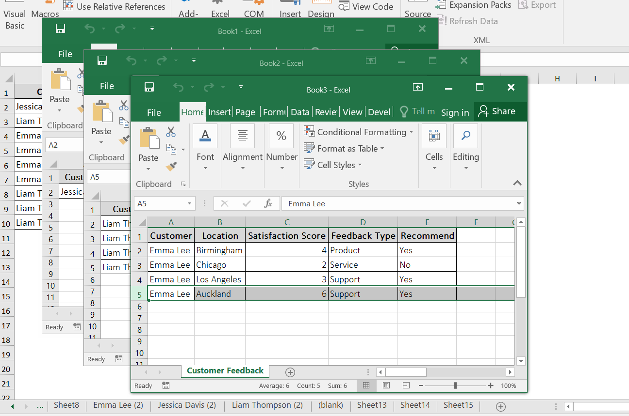
➤ It will split the worksheet into three different files based on column value.
Split Excel Sheets Into Multiple Worksheets Manually
Both processes for splitting the worksheet mentioned above are quite actionable. As for VBA, one downside is that you may need a little technical knowledge, although you can use our script and tweak it according to your project needs.
However, if you are not comfortable with VBA, you can follow one of the two ways.
- Either copy and paste the data manually into the new sheets
- Or, split it while importing the data into Excel (e.g., using Power Query).
Splitting sheets manually is both slow and tedious, especially with larger ones. In such cases, relying on VBA or PivotTable will be far more efficient.
Note:
The Power Query feature is only available in Microsoft 2013 and above versions. If you are not in the category, you have to complete the task using VBA.
Split Excel Sheet By Using Power Query
Now we will split the datasheet into multiple worksheets based on the Customer column value using Power Query. Follow the steps below.
➤ Select your table or data range.
➤ Go to the Data menu >> Select From Table option
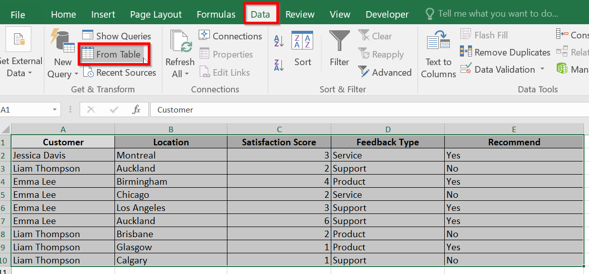
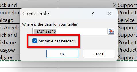
➤ Confirm My table has headers and click OK.
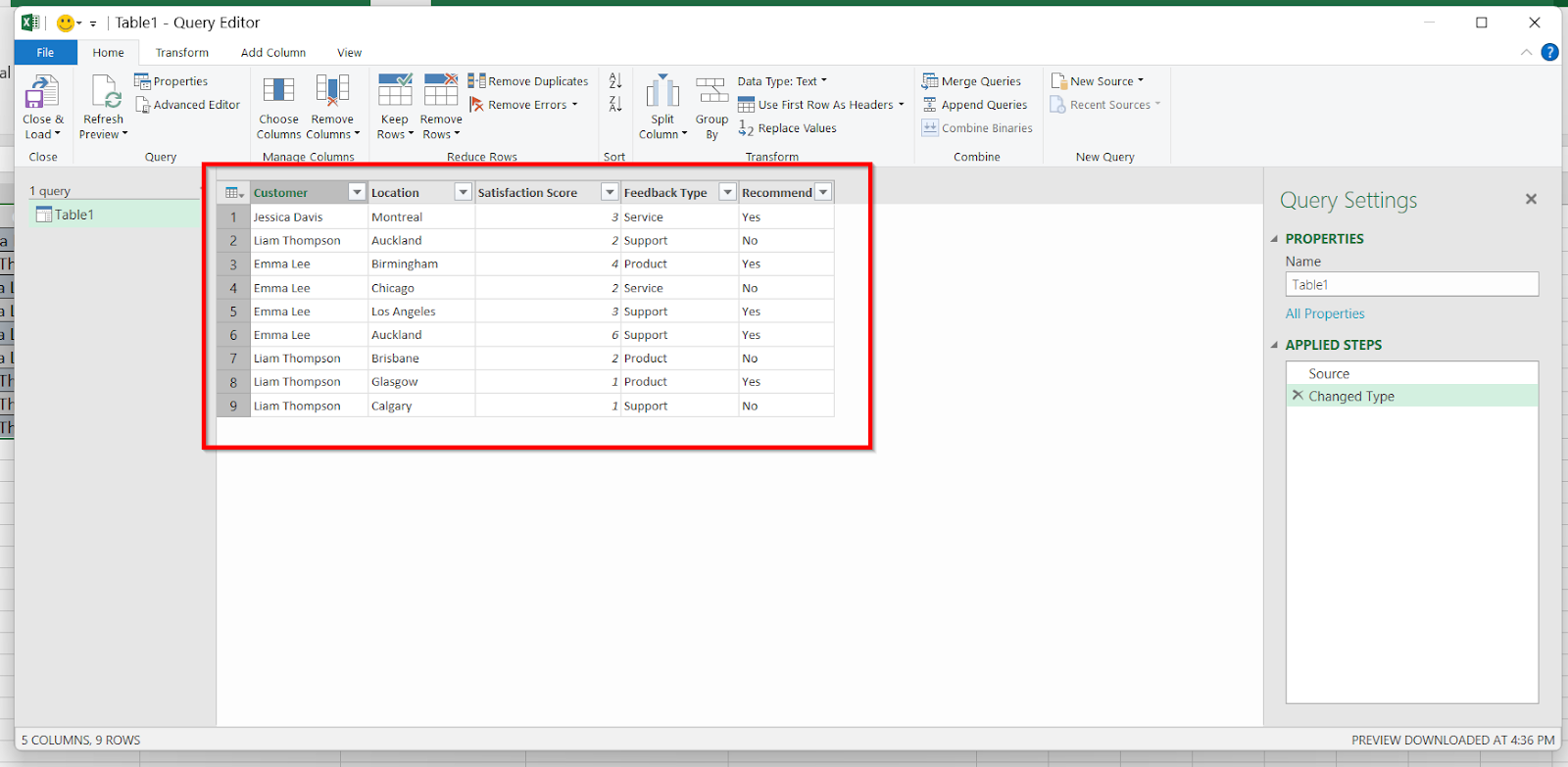
➤ Our data is loaded in Power Query.
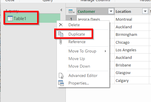
➤ So, now we will duplicate the file. On the left side of the Power Query Editor, select the Table >> Give a right click >> Select Duplicate.
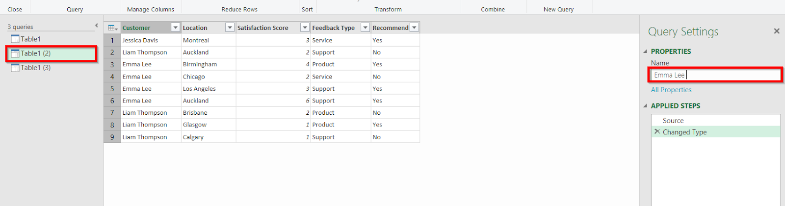
We will have another table. We’ve duplicated two tables for our two customers this time.
➤ We have two different tables for our two different customers.
➤ Now we are just going to rename the Tables. On the right side, under Query Settings, rename based on the data you want to split in the Name field. We have done so based on our customer’s name.
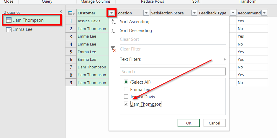
➤ Go into each Table >> Click Filter option.
➤ Choose the name and click OK.
➤ Leave the table as it is and go to the next table. Do the same.
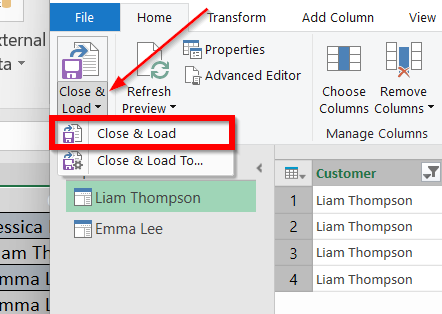
➤ Click on Close & Load >> Select Close & Load.
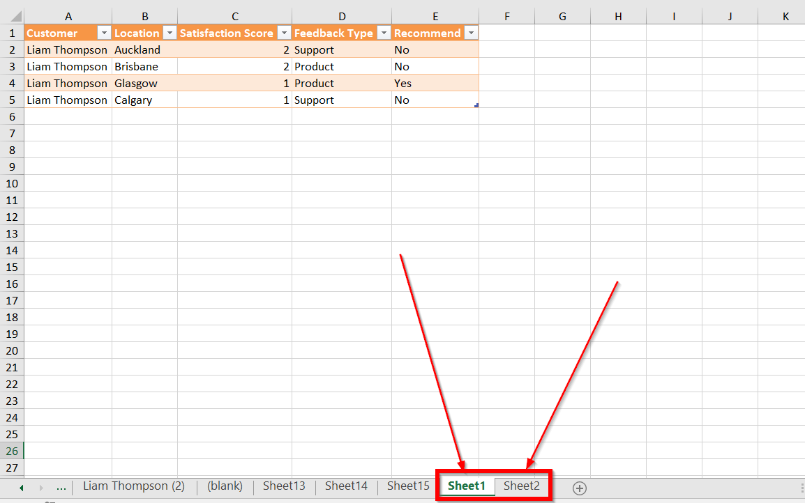
➤ On the Excel sheet, you will see data has been filtered into different sheets.
Frequently Asked Questions
How do I split an Excel sheet into two pages?
- Go to the View tab >> Click Page Break Preview
- Select the row below where you want the page break to occur.
- Go to the Page Layout tab >> Click Breaks
- Select Insert Page Break.
How can I convert multiple individual spreadsheets into one tab on one spreadsheet?
- Open a new blank Excel worksheet
- Click on the Data >> Get Data in the Get & Transform Data section
- Choose From File >> From Workbook. Browse and select your files.
- Select the sheet you want to import in the Navigator window >> Click Load.
- Repeat the steps for each file.
How do you group sheets in Excel?
Press and hold the Ctrl key >> Click on the sheet tabs you want to group. Press and hold the Shift key to group consecutive sheets.
How do I copy data from one Excel sheet to multiple sheets?
- Select the data on the sheet by pressing Ctrl + C .
- Add new worksheets using the plus sign.
- Select the cells in the new worksheet. Press Ctrl + V to paste all the data.
How do you split data in an Excel sheet?
- Go to the Data >> Select Data Tools >> Then Text to Columns
- Select the delimiter to define the place where you want to split the data in the sheet
- Select Apply
Wrapping Up
In this quick tutorial, we have learned the steps to split an Excel sheet into multiple worksheets using three methods. Feel free to download the practice file and let us know which method works out best!