If you’re using Excel for data entry or forms, drop‑down lists are powerful for ensuring consistent, error‑free inputs. But once your list is set up, adding new options can feel rigid. Excel offers multiple ways to add new items to your drop‑down whether you’re working with simple lists, tables, dynamic formulas, or multi-level dependencies.
In this article, you’ll learn step-by-step how to add items to drop-down lists in Excel manually, automatically, or dynamically depending on your version and setup. Whether you’re updating a basic form or managing complex data, these methods help keep your lists flexible and up to date.
Steps to add item to drop-down list in Excel:
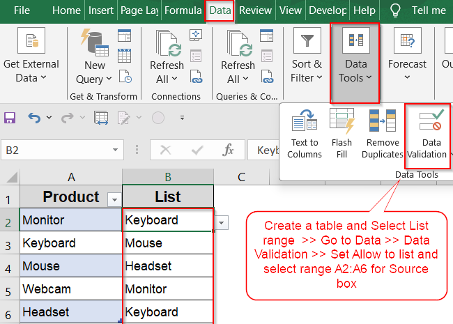
➤ Create a table pressing Ctrl + T .
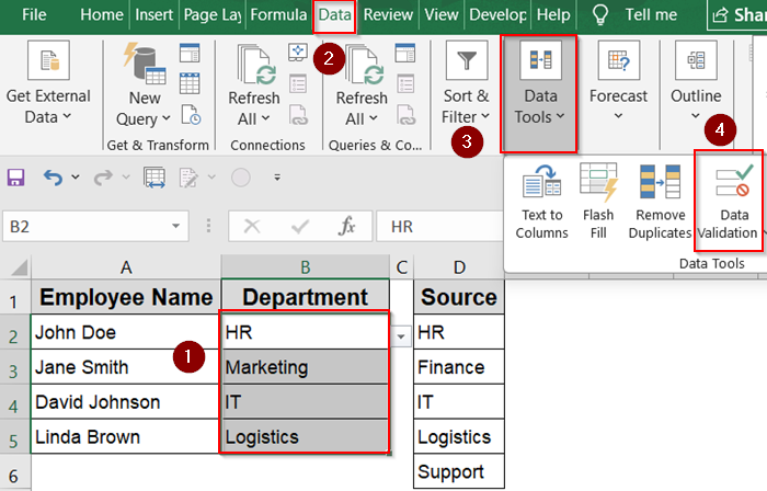
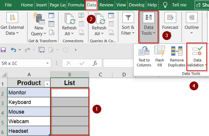
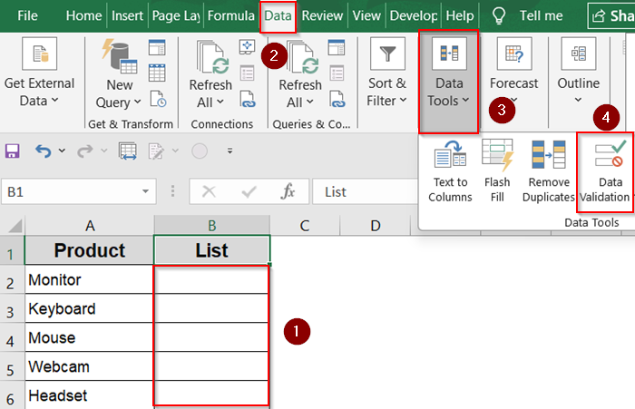
➤ Select the cells such as B2:B6 where the drop-down should appear.
➤ Go to Data >> Data Validation under Data Tools on the ribbon.
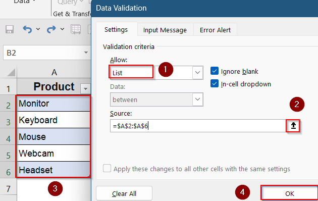
➤ In the Settings tab set Allow to List and select the range A2:A6 or table column using the small button at the left in the Source box.
➤ Click OK.
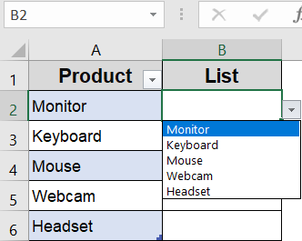
➤ You can now add items below the table column and they’ll appear under the drop-down list automatically.
Edit Source for Fixed Lists Manually
If your drop‑down is based on a fixed range or type‑in list, manually adding items is simple and quick. This method is ideal for occasional updates.
Steps:
➤ Open the worksheet containing your drop‑down source list.
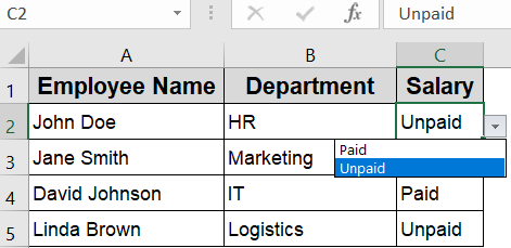
➤ Select range C2:C5 and go to the Data tab >> Data Validation under Data Tools on the ribbon.
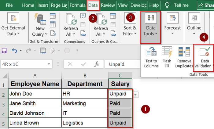
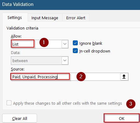
➤ If your list is manually typed and comma separated, then set Allow to List and add new item in the Source box using a comma such as Processing.
➤ Click OK to save.
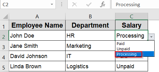
Now you will find your updated drop-down list as you click on the arrow.
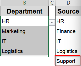
➤ If your existing drop-down is from a fixed source column like column D, add a new item like Support to the next blank cell in the Source column in D6 cell.
➤ Then select your range B2:B5 and go to the Data tab >> Data Validation under Data Tools.
➤ You will see your range in the Source box.
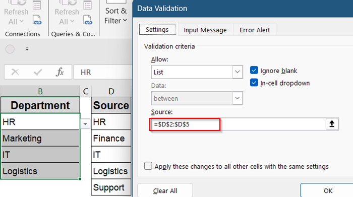
➤ To update your source, edit the range to =$D$2:$D$6 from =$D$2:$D$5 and click OK.
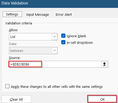
Now your drop-down has been updated in the Department column.

Use an Excel Table for Dynamic Auto‑Updating
This is the fastest way to build a drop-down list from a column of values. When you convert a range into an Excel Table, the drop-down list updates automatically as you add more items which is perfect for structured, frequently updated datasets.
Steps:
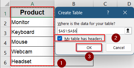
➤ Turn your source data A2:A6 into a Table using Ctrl + T and check your headers. Then, click OK.
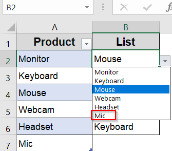
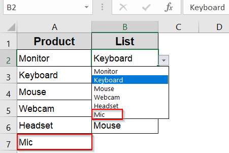
➤ If you have an existing drop-down list, you can add data below your table source such as Mic in column Product and check your existing drop-down List column by clicking on the drop-down arrow.

➤ However, if you do not have a pre-existing drop-down list created, select the cells such as B2:B6 where the drop-down should appear.
➤ Go to Data >> Data Validation under Data Tools on the ribbon.
➤ In the Settings tab set Allow to List and select the range A2:A6 or table column using the small button at the left in the Source box.
➤ Click OK.
➤ You will find a drop-down arrow next to the selected cells using your Table data as the source.
Now, you can add each new item simply below the table and Excel will auto-expand it and update the drop‑down list instantly such as Mic in A7 cell.
Extend Existing Named Range
If you have a specific named range in your data that you used as the source for your drop-down list and now you want to add items to your drop-down, then this method is for you. You can update your named range very easily which will instantly reflect on your drop-down list column.
Steps:
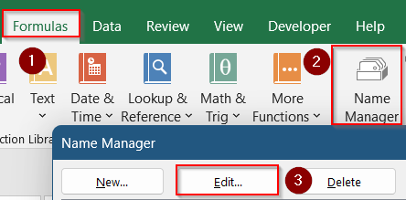
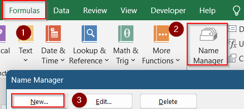
➤ To edit an existing named range such as SourceList, go to Formulas >> Name Manager >> Click Edit.
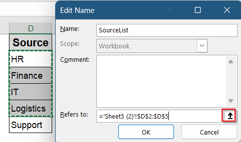
➤ After that, click the small arrow button in the Refers to box to add a new item.
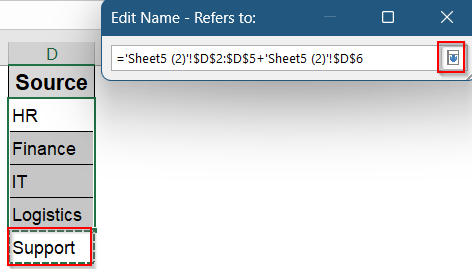
➤ Then just click on the cell you wish to add such as Support in D6 cell and click the arrow button to go back and click OK.
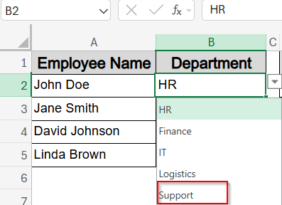
You will see that your drop-down list has updated automatically.
Define Dynamic Range with OFFSET Function
For versions before dynamic arrays or when working with manual ranges, the OFFSET function enables dynamic lists that grow automatically when items are added. By using this method, you can avoid any extra steps needed later on for adding items to your drop-down list.
Steps:
➤ Suppose your list starts at Sheet3!A2.
➤ Click Formulas tab >> Go to Name Manager on the ribbon >> Click New.
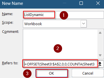
➤ Give it a Name it such as ListDynamic.
➤ In Refers to box, enter:
=OFFSET(Sheet3!$A$2,0,0,COUNTA(Sheet3!$A:$A)-1,1)
➤ Click OK.
➤ Close the Name Manager dialog box.
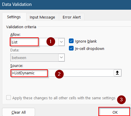
➤ Go to Data >> Data Validation under Data Tools on the ribbon.
➤ In the Settings tab, set Allow to List and in the Source box type:
=ListDynamic
➤ Click OK.
Your drop-down list will now grow or shrink automatically when you update the source list such as we added Mic in A2 cell and it appeared in the drop-down instantly.
Apply UNIQUE Spill Formulas (Excel 365/2021)
With modern Excel, you can extract a unique, dynamic list with UNIQUE function and directly reference its spill range in Data Validation.
Steps:
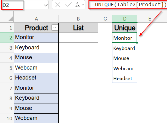
➤ Suppose your table column is A2:A14.
➤ In an empty cell (e.g. D2), enter:
=UNIQUE(Table2[Product])
➤ The list spills down populated values.
➤ Select range B2:B6 >> Go to Data >> Data Validation under Data Tools on the ribbon.

➤ In the Settings tab, set Allow to List and in the Source box type
=$D$2#
➤ Click Apply to save changes.
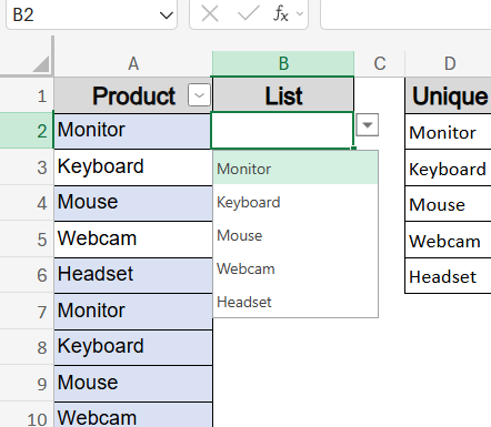
This drop-down always shows unique entries and updates as the source table changes.
Frequently Asked Questions
How do I add an item in Excel drop-down?
To add items in Excel drop down, update the source range or table. For dynamic lists, functions like UNIQUE auto-update while static lists need manual source changes.
What if the drop‑down doesn’t expand when I add new items?
If you’re using a standard table, ensure the table auto‑expands. For named ranges or OFFSET formulas, verify the definitions include the new items correctly.
Can I allow users to enter items not in the list?
Yes. In Data Validation settings, deselect “Show error alert after invalid data is entered” to allow free typing beyond the drop-down.
Wrapping Up
In this tutorial, we explored several ways to add items to drop‑down lists in Excel that match your workflow. Whether you need simplicity or flexibility, use manual edits for small lists, Tables or UNIQUE function for dynamic updates or OFFSET function for legacy versions. Feel free to download the practice file and share your feedback.