If you’re working with large datasets in Excel, spotting incorrect entries manually can be time-consuming and error-prone. Luckily, Excel provides a built-in Circle Invalid Data feature that visually flags entries that don’t meet your validation rules. It’s especially helpful when enforcing number limits, drop-down selections, or formatting standards.
In this article, you’ll learn how to use the Circle Invalid Data tool, add input guidance for users, set up custom error alerts, and apply alternative methods like conditional formatting and formulas. These approaches help you ensure cleaner data, reduce manual checks, and build smarter spreadsheets.
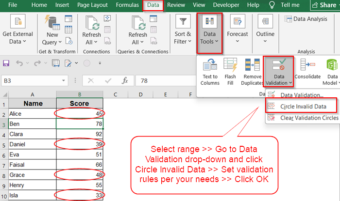
Steps to circle invalid data in Excel:
➤ Select the range of cells you want to check such as A2:A10.
➤ Go to Data >> Data Validation under Data Tools group.
➤ In the dialog box, under the Settings tab, set your validation rule. For example, set Allow to Whole number, Data to greater than or equal to and type 50 in Minimum.
➤ Click OK to apply the rule and click on Data Validation dropdown and select Circle Invalid Data.
Use 'Circle Invalid Data' Option from Data Validation
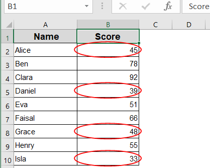
This method is the fastest way to visually flag invalid entries. Excel will automatically draw a red circle around any cell that doesn’t comply with your set validation rules. This is especially useful when you’re working with numerical thresholds, allowed lists, or specific formats.
Steps:
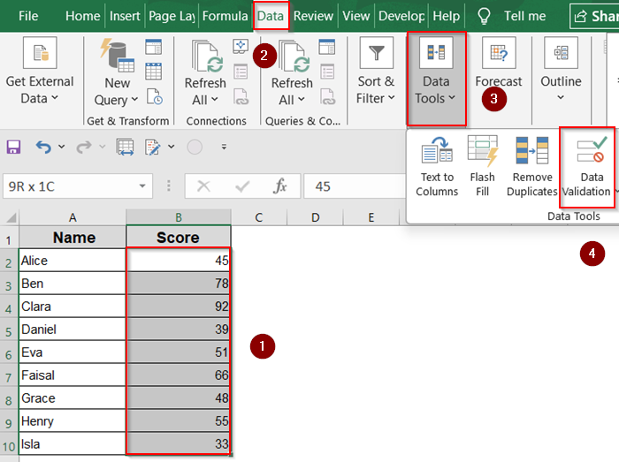
➤ Select the range of cells you want to check such as A2:A10.
➤ Go to the Data tab.
➤ Click the Data Validation dropdown (in the Data Tools group).
➤ Choose Data Validation.
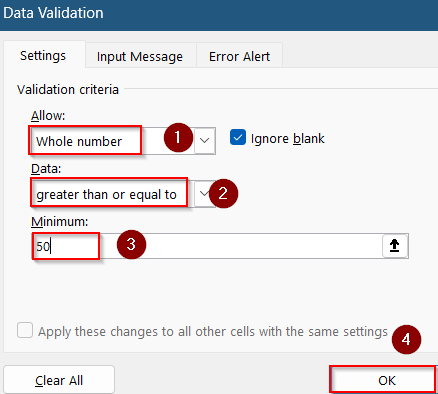
➤ In the dialog box, under the Settings tab, set your validation rule. For example, set Allow to Whole number, Data to greater than or equal to and type 50 in Minimum. You can choose other options based on your requirements.
➤ Click OK to apply the rule.
➤ Go back to the Data Validation dropdown.
➤ Click Circle Invalid Data.
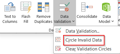
Red circles will now appear around any values in the selected range that don’t meet your criteria.
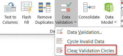
➤ To remove the red circles, return to the same menu and click Clear Validation Circles.
Add Input Message for Entry Guidance
Instead of only reacting to invalid entries, you can proactively guide users with input messages. Excel’s Data Validation allows you to display a custom message when a user selects a cell. This message can describe what’s expected such as allowed ranges or formats and helps reduce mistakes before they happen. It’s a simple but effective way to improve user experience and avoid repeated corrections.
Steps:
➤ Go to Data >> Data Validation under Data Tools group.

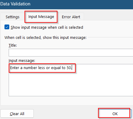
➤ Click on the Input Message tab.
➤ Type a helpful message like “Enter a number less or equal to 50”.
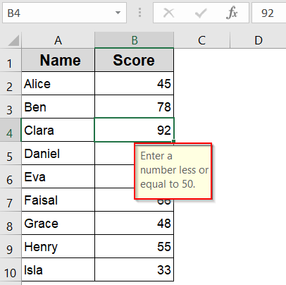
Now, if we click on B4 cell, this appears as a tooltip when the cell is selected which is a proactive guide to reduce mistakes.
Customize Error Alert Type
When users enter something that breaks your validation rules, Excel can trigger an error alert. Depending on how strict you want to be, the alert can block the entry, display a warning, or simply inform the user. By customizing the message and style, you can control how Excel handles invalid inputs.
Steps:
➤ Go to Data >> Data Validation under Data Tools group.

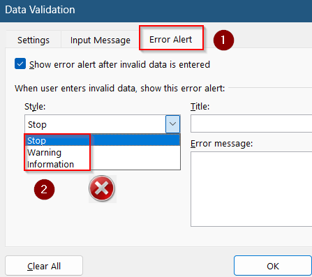
➤ Click on Error Alert tab.
➤ You can choose Stop to block the entry completely, Warning to show a message but allows the user to override and Information to notify the user but always accepts input.
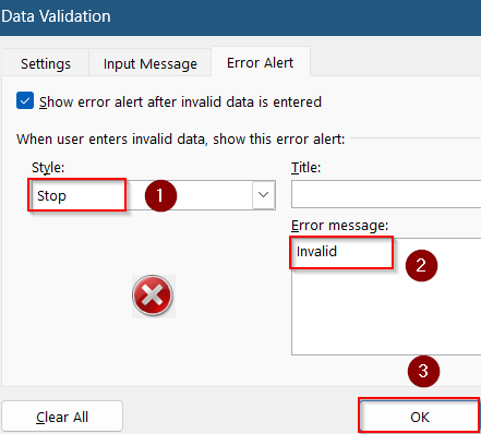
➤ For example, set the Style to Stop and adding Invalid as the Error message. Then, click on OK.
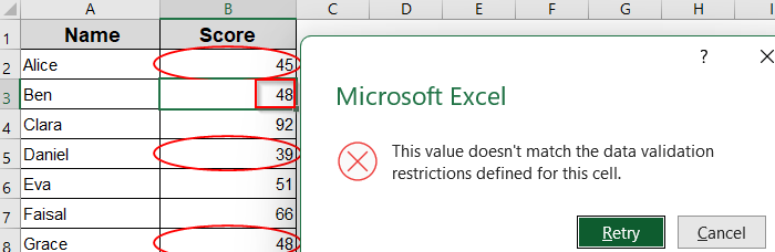
Now we will see an error pop-up from the system whenever invalid entries are attempted such as 48 in this case.
Apply Conditional Formatting to Highlight Invalid Cells
This method is ideal when you want to use colors or styles instead of circles. Conditional formatting lets you highlight invalid values using rules that update dynamically as data changes.
Steps:
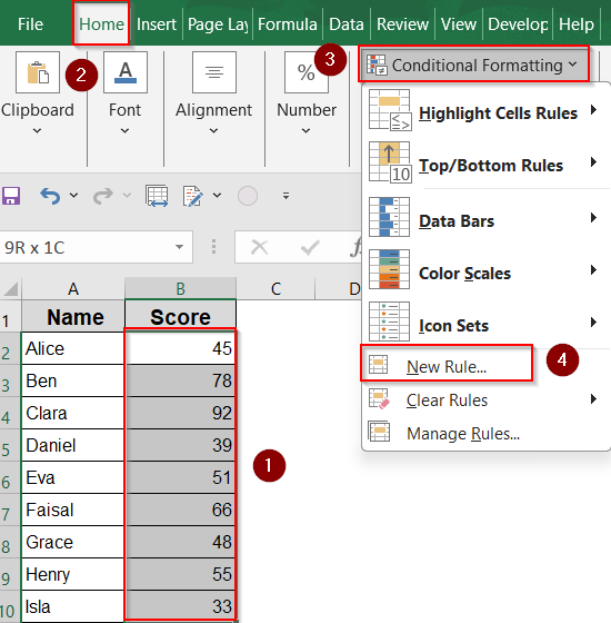
➤ Select the range you want to validate (e.g., A2:A10).
➤ Go to the Home tab.
➤ Click Conditional Formatting >> New Rule.
➤ Choose Use a formula to determine which cells to format.
➤ Enter a formula like this:
=B2<50
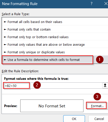
➤ Click Format, then choose a fill color such as orange to apply.
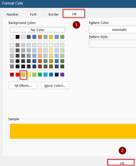
➤ Click OK, and then click OK again.
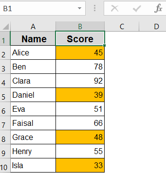
Any cell with a value less than 50 will now be highlighted based on your formatting preferences. This method works in real-time and is more flexible than red circles.
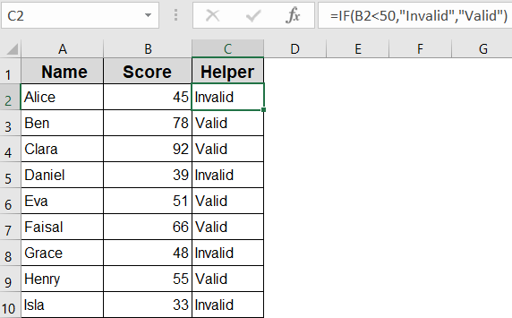
Insert a Custom Formula in a Helper Column
This method is best when you need a simple “Valid/Invalid” label beside each value without relying on visual formatting. It’s useful for exporting or filtering results.
Steps:
➤ Insert a new column next to your data (e.g., column C next to column B).
➤ In cell C2, enter this formula:
=IF(B2<50,”Invalid”,”Valid”)
➤ Press Enter, then drag the fill handle down to apply the formula to other rows.
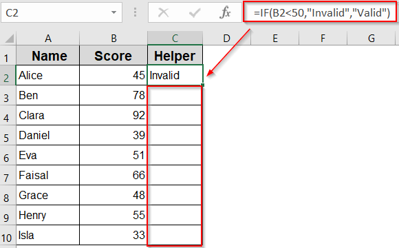
Now, you’ll see either Valid or Invalid in column B for each row. You can filter or sort by these results to group similar entries together.
Frequently Asked Questions
Why do the red circles disappear when I save or re-open the file?
The red circles from Circle Invalid Data are visual aids, not permanent formatting. Excel clears them when the file is saved or reopened, so you’ll need to manually reapply them.
Can I print the sheet with the red circles visible?
No, the circles are only for on-screen viewing. They help during data review but won’t appear in printouts or exported PDFs, so use conditional formatting if print visibility is required.
What happens if I use both Conditional Formatting and Circle Invalid Data?
You can use both together. Conditional formatting applies color or styling, while Circle Invalid Data adds visual rings. They won’t interfere with each other but are managed separately in the interface.
Is there a way to make Circle Invalid Data update automatically?
Not natively. The feature doesn’t refresh automatically with new inputs or changes. While you can try VBA, it’s often unreliable which is why conditional formatting is a better real-time alternative.
Wrapping Up
In this tutorial, we learned multiple ways to identify and highlight invalid data entries in Excel. From using the Circle Invalid Data feature for instant visual cues to applying conditional formatting, error alerts, and helper column formulas, each method serves a different purpose depending on your workflow. Feel free to download the practice file and share your feedback.