Counting unique values in Excel is a common task for data analysis, but things get a bit more complex when you need to apply multiple criteria. Whether you’re tracking unique customers by region and product or filtering unique transactions by date and status, Excel offers several methods to count unique values dynamically and accurately. Mastering these techniques will help you generate insightful reports and dashboards with ease.
In this article, you’ll learn the best methods to count unique values in Excel with multiple criteria. We will cover formula-based methods, built-in tools and coding solutions for automation. Each approach works well depending on your Excel version and the complexity of your dataset.
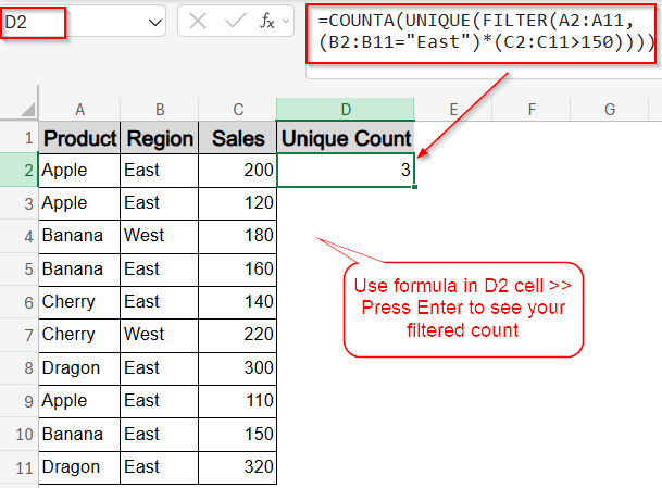
Steps to count unique values in Excel with multiple criteria:
➤ Go to a blank cell like D2 where you want your output to show.
➤ Use this formula:
=COUNTA(UNIQUE(FILTER(A2:A11,(B2:B11=”East”)*(C2:C11>150))))
➤ Press Enter.
Count Unique Values with FILTER, UNIQUE, and COUNTA Function (Excel 365 / 2021)
This method uses Excel 365’s dynamic arrays to filter rows based on multiple criteria, then counts distinct values in a single column. It’s clean, readable, and perfect for column-based uniqueness.
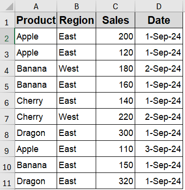
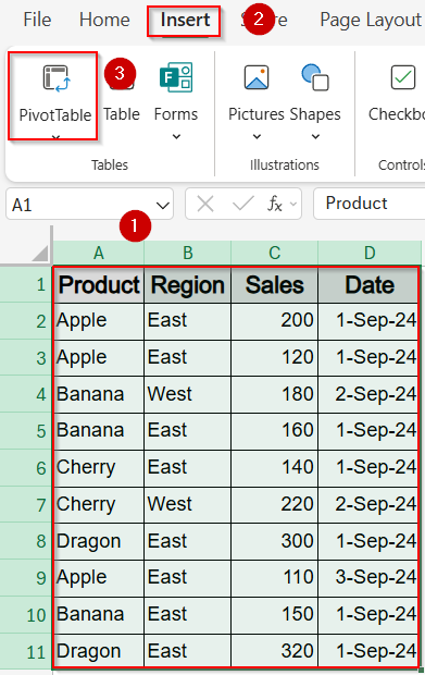
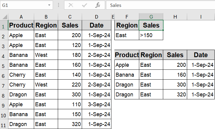
In this example, our sample dataset tracks product sales by region and date. We’ll extract entire rows that match specific criteria like Region = “East” and Sales > 150 using formulas that return all matching records, not just one value.
Steps:
➤ Go to a blank cell like E2 where you want your output to show.
➤ Use this formula:
=COUNTA(UNIQUE(FILTER(A2:A11,(B2:B11=”East”)*(C2:C11>150))))
Change A2:A11 to the column you want to count; update B2:B11 and C2:C11 to your filter columns and criteria.
➤ Press Enter.
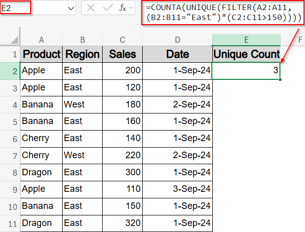
It returns the count of unique product names in the East region with sales over 150.
Combine FREQUENCY with MATCH Function to Count Unique Values
This method calculates unique values using a combination of functions like MATCH, FREQUENCY, and array logic, making it compatible with older Excel versions that don’t support dynamic arrays or FILTER.
Using this technique returns the number of unique products sold in the East region on September 1, 2024, based on the dataset. The result helps you quickly identify how many distinct products meet these specific criteria without listing each one individually.
Steps:
➤ Use this array formula in E2 cell:
=SUM(–(FREQUENCY(IF((B2:B11=”East”)*(D2:D11=DATE(2024,9,1)),MATCH(A2:A11,A2:A11,0)),ROW(A2:A11)-ROW(A2)+1)>0))
Change A2:A11 to your target column, and adjust B2:B11 and D2:D11 with your Region and Date columns or values.
➤ Press Ctrl + Shift + Enter for older Excel versions and only Enter for modern Excel versions.
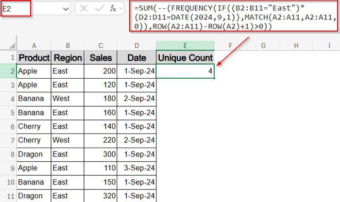
This counts how many unique products were sold in the East region on 01-Sep-24.
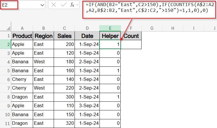
Use a Helper Column and COUNTIFS Function
This approach creates a helper column to track first occurrences of values that match multiple conditions. It’s especially helpful for clearly identifying and counting unique products sold in a specific Region like East with a minimum Sales value like 150 in your dataset.
Steps:
➤ In E2 (helper column), insert:
=IF(AND(B2=”East”,C2>150),IF(COUNTIFS(A$2:A2,A2,B$2:B2,”East”,C$2:C2,”>150″)=1,1,0),0)
Update A2, B2, and C2 with your data columns and criteria; use the same structure for different logic.
➤ Press Enter and drag down to E11.
➤ Then, use this formula in F2 cell:
=SUM(E2:E11)
Adjust E2:E11 if your helper column is placed in a different range.
➤ Press Enter.
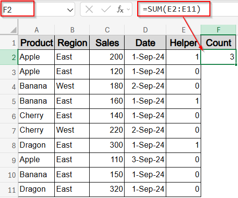
This method is excellent for troubleshooting and manual checking.
Count Unique Values Combining IFERROR and ROWS Functions
In this method, the ROWS function counts the number of rows in a range, while the IFERROR function handles any errors by replacing them with blanks. Together, they count only the valid unique values returned by a formula without interruption.
When applied to the dataset, this method returns the total count of unique products sold in the your chosen region such as East with sales over 150, handling any missing matches neatly for an accurate count.
Steps:
➤ Use this formula in E2 cell:
=IFERROR(ROWS(UNIQUE(FILTER(A2:A11,(B2:B11=”East”)*(C2:C11>150)))), 0)
Change A2:A11 to the unique column and B2:B11, C2:C11 to the filter columns and condition values.
➤ Press Enter.
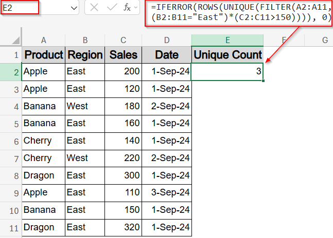
It counts the number of unique products where Region is set to East and Sales is greater than 150.
Count Unique Values Using SUMPRODUCT with COUNTIFS
In this method, the COUNTIFS function checks how many times each value appears while applying specific conditions. When you divide 1 by that result, duplicates contribute fractional values. SUMPRODUCT function adds those fractions to return the total number of unique values that meet the given criteria. This method is reliable even in Excel versions that don’t support dynamic array functions like UNIQUE.
The formula checks if dates in column D are equal to 1-Sep-2024, filters rows where Region is set to “East,” and counts unique values in A2:A11 meeting both criteria.
Steps:
➤ Go to a blank cell like E2.
➤ Use this formula:
=SUMPRODUCT((B2:B11=”East”)*(D2:D11=DATE(2024,9,1))*(1/COUNTIFS(A2:A11,A2:A11,B2:B11,”East”,D2:D11,DATE(2024,9,1))))
Modify A2:A11 to the column you’re analyzing, and adjust Region/Date columns and conditions as needed.
➤ Press Enter.
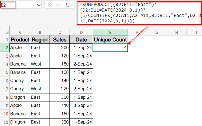
Now you have your unique count based on multiple criteria.
Try Distinct Count with PivotTable
Using a PivotTable lets you quickly summarize large datasets by grouping and analyzing data. To count distinct values, you add the desired field (like Product) to the Values area and set the calculation to “Distinct Count.”
Excel then scans the dataset, filters out duplicates within each group (such as Region or Date), and returns the total number of unique entries. This method is especially useful when you want to break down unique counts across categories without writing any formulas.
Steps:
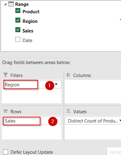
➤ Select range A1:D11 and go to the Insert tab >> Click PivotTable
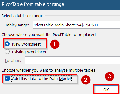
➤ Select New Worksheet >> Check the box for Add this data to the Data Model and click OK.
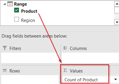
➤ Now drag Product to the “Values” field.
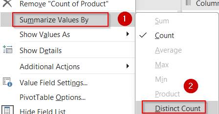
➤ Right-click the count number inside the PivotTable and choose Summarize Values By >> Distinct Count.
➤ Add Region to the Filters area and Sales to the Rows area.
➤ Right-click Row Labels >> Set Label Filters to Greater than and type 150 >> Click OK.
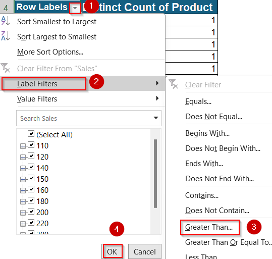
➤Then set the Region to filter by the East region only.
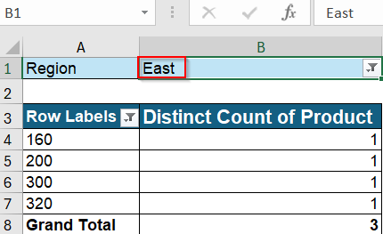
Now you have your total count of unique values greater than 150 in the East region displaying each value for better visualization.
Count Unique with Advanced Filter and ROWS Formula
Advanced Filter is a built-in Excel feature that copies unique rows matching your criteria to a new location without formulas. Using ROWS function on this filtered output counts the unique records dynamically and simply.
This method returns a list of unique products from the dataset such as those sold in the East region with sales over 150 along with the exact count of these distinct products, clearly showing how many meet your filter conditions.
Steps:
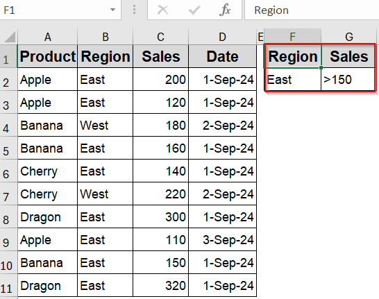
➤ Add two new columns called Region and Sales in column F and G respectively.
➤ Place filter values like East and >150 in F2 and G2 cells.
➤ Go to the Data tab >> Click Advanced from the Sort & Filter group.
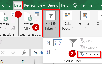
➤ Select Copy to another location and list your original range A1:D11 using the small arrow button at the right.
➤ Set Criteria range as F1:G2 which is our customized filter area.
➤ Under Copy to, select the cell from where you want your output to show such as F4 cell.
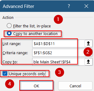
➤ Click OK and your output will spill automatically that matches your filters ranging from F4:I8.
➤ Then, enter this formula to display total count in a blank cell like F11:
=ROWS(F5:I8)
Change F5:I8 to match the output range where your filtered results appear (excluding the header). This returns a count of unique rows matching the filter.
➤ Press Enter.
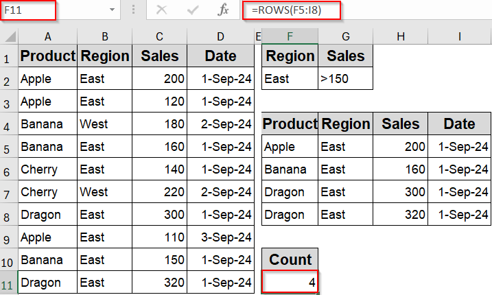
Now you will find 4 as your total count displaying for relevant filters like East as Region and Sales greater than 150.
Count Unique Values with VBA User-Defined Function (All Excel Versions)
This method uses a custom VBA function to count unique values based on multiple criteria. While a formula is still required, coding avoids helper columns and supports deeply nested logic. It also works across all Excel versions.
This returns the number of unique values in column A (like Product) where Region is East and Sales greater than 150 when you run the code and use a formula in the output cell.
Steps:
➤ Press Alt + F11 to open the Visual Basic for Applications (VBA) editor.
➤ Go to Insert >> Module, and paste the following code:
Function CountUniqueWithCriteria(rngData As Range, rngRegion As Range, rngSales As Range, _
                                 criteriaRegion As String, criteriaSales As Double) As Long
    Dim dict As Object
    Set dict = CreateObject("Scripting.Dictionary")
    Dim i As Long
    For i = 1 To rngData.Rows.Count
        If rngRegion.Cells(i, 1).Value = criteriaRegion And rngSales.Cells(i, 1).Value > criteriaSales Then
            If Not dict.exists(rngData.Cells(i, 1).Value) Then
                dict.Add rngData.Cells(i, 1).Value, 1
            End If
        End If
    Next i
    CountUniqueWithCriteria = dict.Count
End Function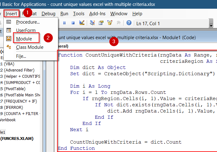
➤ Close the VBA editor (Alt + Q), return to your sheet, and enter this formula in F2 cell:
=CountUniqueWithCriteria(A2:A11, B2:B11, C2:C11, “East”, 150)
Adjust A2:A11 to your unique column; change B2:B11, C2:C11, and the “East“, 150 inputs as needed.
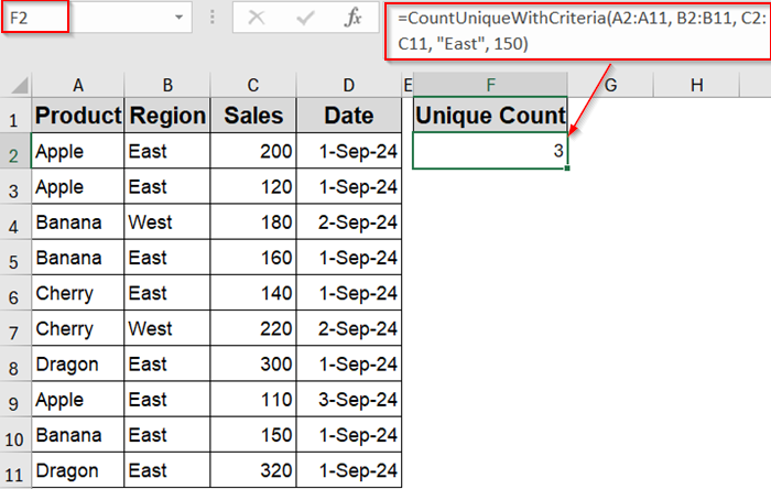
Now your data count is visible based on set criteria.
Frequently Asked Questions
Can I count unique values with multiple criteria in Excel versions before 365?
Yes, you can use legacy formulas like SUMPRODUCT with COUNTIFS or FREQUENCY with MATCH function, which work in older versions without dynamic array functions used in modern Excel versions.
How do I handle blank or error cells in unique counts?
Wrap your formulas with IFERROR function or filter out blanks using FILTER function to ensure accurate counts without errors or empty cells affecting results.
Can I count unique values across multiple columns with multiple criteria?
Yes. By filtering entire rows and then using functions like UNIQUE with ROWS or by combining helper columns, you can count distinct full-row entries based on multiple conditions.
Is there a way to count unique values visually without formulas?
Using PivotTables with the Data Model allows you to count distinct values interactively without writing formulas which works best for dashboard reports.
Wrapping Up
In this tutorial, we learned several effective methods to count unique values in Excel with multiple criteria, ranging from dynamic array formulas to legacy array functions and built-in tools like PivotTables, Advanced Filter, and VBA. Each method has its strengths and works best depending on your Excel version and suitable needs, helping you analyze data efficiently and accurately. Feel free to download the practice file and share your feedback.