Discount rates are a common metric in financial calculations. If you are investing an amount of money for a certain period of time, you might want to know the interest rate you are going to receive for that money. In Excel, there are a bunch of ways to calculate the discount rate. In this article, we will learn all of the ways with a step-by-step guide so that you can learn how to calculate the discount rate in Excel with ease.
➤ Use the following formula to calculate the discount rate:
=RATE(C2,0,-A2,B2)
➤ Replace C2 with the number of periods (n), A2 with the present value (PV), and B2 with the future value (FV).
➤ If you have multiple calculations in your table, autofill other cells.

That was one method to do the discounting. But, there are a lot of other ways to calculate discount rates as well. Read the whole article to understand all of the methods.
Calculating Simple Discount Rate
When you invest a one-year amount of money and receive a larger amount afterwards, we can calculate the discount rate using this method. Even without considering the financial aspects, say that you are buying something from a shop. The shopkeeper is giving you some dollars off, but you want to know the discount rate. This method will help you calculate that as well.
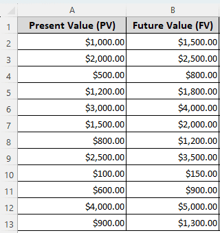
We have a table of just present values and future values for this calculation. If you are doing discount rates for shopping, you will have to replace them with the current price and the future price, respectively. Let’s get to the calculation:
➤ Create a new column for the Discount Rate (Calculated). We are choosing the C column.
➤ Insert any of the following formulas in the C2 cell.
=-(1-(B2/A2))
=(B2-A2)/A2
➤ Click on the C2 cell again, and select the percentage (%) sign from the Number group of the Home tab.
➤ Autofill other cells in the column.
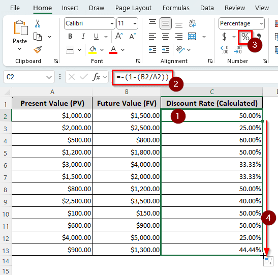
In the second formula, we just divide the difference between the future and present value by the present value to get the discount rate.
Finding the Discount Rate from Multiple Periods
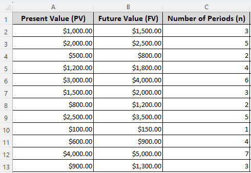
In most financial investments, you will receive the future value after a certain period of time, also known as the maturity period. When you have multiple periods to account for, you should use the current method. We are using the previous dataset for this, but we added another column for the number of periods to help calculate the discount rate.
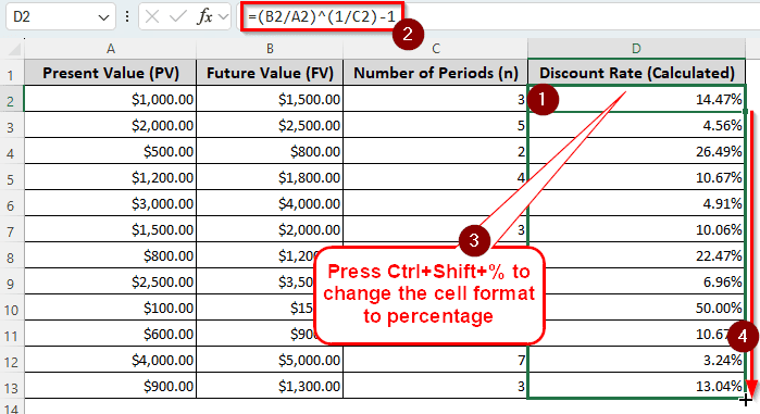
➤ Like the previous method, add a new column for the discount rate calculation. We are going for the D column with the heading “Discount Rate (Calculated)”.
➤ Write this formula in the D2 cell:
=(B2/A2)^(1/C2)-1
➤ After pressing Enter, the formula will work, but the cursor will move on to the D3 cell. Go back to the D2 cell and press Ctrl+Shift+% to change the cell formatting to percentage.
➤ Drag the bottom-right of the D2 cell to the D13 cell to autofill the column.
=((FV/PV)^(1/n) ) - 1
Here, the FV is B2, the PV is A2, and n is C2.
Using the RATE Function to Get the Discount Rate from Multiple Periods
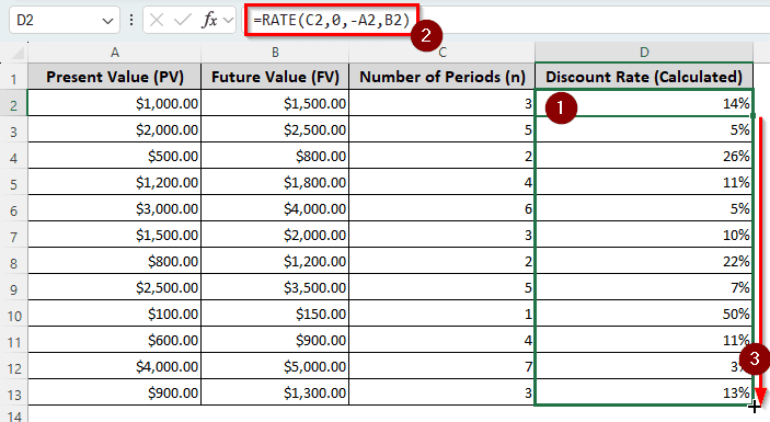
Instead of using regular mathematical calculations, we can use a function provided by Microsoft Excel itself. The function is called RATE, and it gives the discount rate from a few parameters. Let’s use this function:
➤ In the helper column, write the following formula in the first cell after the heading:
=RATE(C2,0,-A2,B2)
➤ Autofill other cells in the column.
Utilizing What-If Analysis with the FV Function
Excel can automatically find a value based on another value if we use a formula to calculate the first value. Confused? Keep reading.
We have inserted the present value and the number of periods in our data range. We will insert the discount rate based on a guess and the future value using a formula. Then we will ask Excel to change the discount rate according to our desired future value. Let’s start:
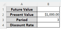
➤ In the B4 cell, write 0.10 / 10%. That is our guessed discount rate.
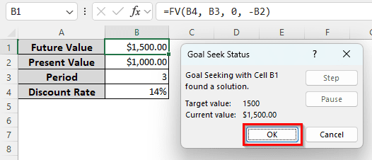
➤ In the B1 cell, write the following formula for the future value:
=FV(B4, B3, 0, -B2)
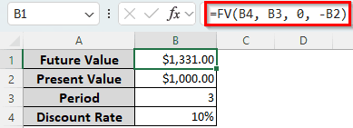
➤ We want to calculate the discount rate when the future value is $1500.
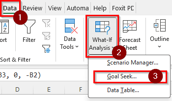
➤ Go to the Data tab, locate the Forecast group, and select What-If Analysis > Goal Seek.
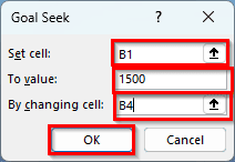
➤ In the Goal Seek window, change the values to the following:
Set cell: B1
To value: 1500
By changing cell: B4
➤ Press OK and wait for the calculation to be done. After it completes, press OK again to see the result.
Frequently Asked Questions
What is a discount rate in NPV?
When you invest in something, you want to know if there are other investment opportunities with better output. The discount rate in NPV provides the rate you will receive when you invest in an alternative opportunity.
What is a 10% discount rate?
It means that the amount of returns you will receive in the future years will have to be reduced by 10% in order to match the present value of money.
How to calculate 10 percent?
You need to multiply the base amount by the percentage. Here is an example with Excel:
=A1*(10/100)
Here, A1 is the base amount.
How to calculate the discount price?
You have to subtract the discounted amount from the listed price. The formula in Excel can be written like the following:
=A1-B1
Replace A1 with the listed price and B1 with the discounted amount.
How to calculate a discount?
Multiply the discount rate by the price of the product. In Excel, the formula will be like the following:
=A1*0.20
Here, A1 is the price of the product, and 0.20 indicates a 20% discount.
Wrapping Up
In this article, we have learned all the ways you can calculate the discount rate in Excel. Feel free to download the workbook we used in this tutorial to practice the methods yourself. Leave your feedback below for us, and we will see you in another tutorial.