How to Add a Comma Between Names in Excel (8 Different Ways)

You may have a list of names in the same cell, or different columns/rows, and want to add a comma between the names in just a few clicks. Excel allows you to automate the process using its intuitive tools and combination of functions.

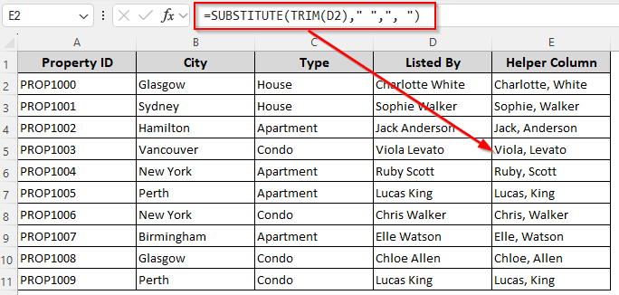
To add a comma between two names in the same cell, we can use a formula with the SUBSTITUTE and TRIM functions. It replaces the space between the two names with a comma and a space.

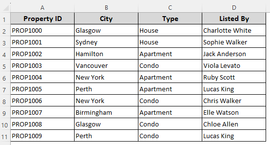
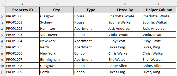
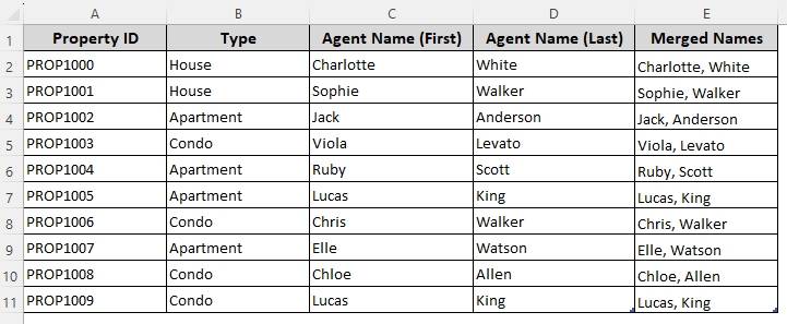
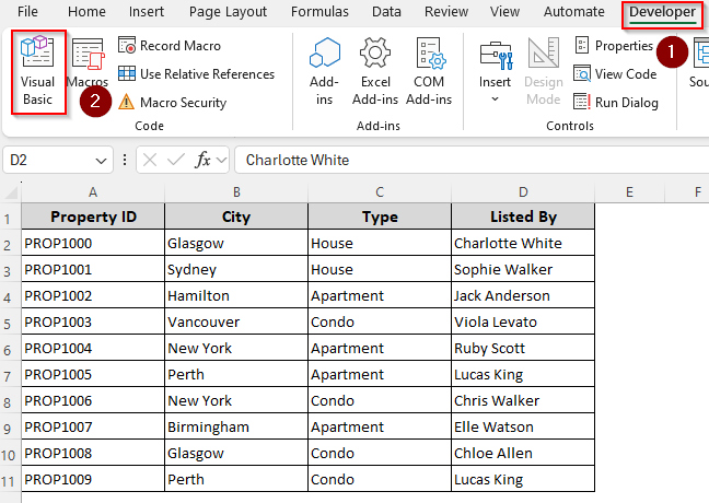
In our dataset, we have columns for real estate listings and related details. Column D includes the first and last names of the listing agents. Our goal is to separate the names with a comma.

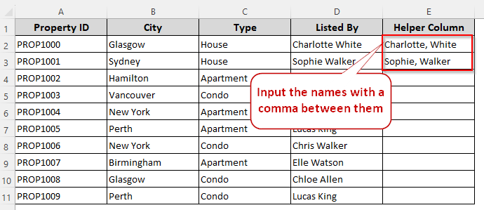
Excel’s Flash Fill feature recognizes patterns and makes changes in the data based on the patterns. So, we’ll manually input the outcome we want and use Flash Fill to change the data from the remaining cells. Here are the details:

➤ Create a helper column and manually input the names with a comma in the first two cells.

➤ Now, select these two cells and the remaining cells that you want to fill and press  CTRL  +  E  .
➤ Or, go to the Data tab and click on the Flash Fill icon from the Data Tools group.

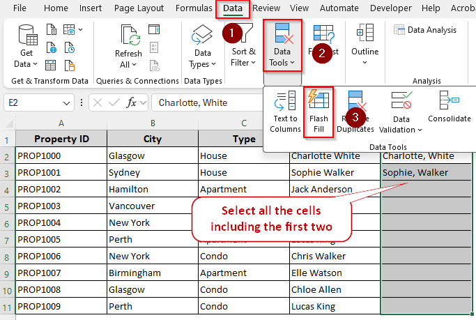
➤ Excel will now add a comma between the names in the remaining cells.

Before you use this method, make sure there are no extra spaces in the cells except for the one between the names. We’ll use the Find & Replace tool to replace the space between two names with a comma followed by a space. Below are the steps:

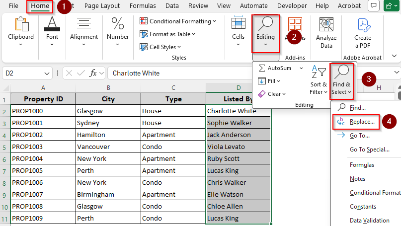
➤ Select the cell range with the names and go to the Home tab. Click on the Find & Select option in the Editing group.
➤ From the drop-down menu, choose Replace.

➤ As the Find and Replace dialog box appears, type a space in the Find What field.
➤ In the Replace With field, type a comma and a space.

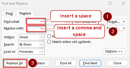
➤ Finally click on Replace All and press Close once the replacement is done. Our final result is as follows:

Excel’s SUBSTITUTE function replaces specific text in a cell with new text. Whereas, the TRIM function removes extra spaces from text, leaving just single spaces between words. We’ll combine these two functions to replace the space between two names with a comma followed by a space. Let’s get to the steps:

➤ In a helper column cell, enter the following formula:

➤ Change the cell reference D2 with your source’s reference containing the names you want to separate by a comma.
➤ Click Enter and use the fill handle (+ sign on the bottom corner of the cell) to autofill the remaining cells.

If you only have two names separated by a space in a cell, you can use the REPLACE and FIND functions to add a comma. However, our formula will replace only the first space with a comma, so it won’t work for more than two names.

While the FIND function locates the position of the first space in a cell, the REPLACE function will insert a defined character (a comma) at that position. Here are the steps:

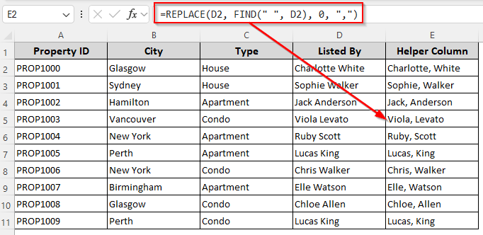
➤ Insert the following formula in a helper column cell:

➤ Instead of D2, enter the cell reference from your data containing the names.
➤ Click Enter and drag the formula down to separate names in the rest of the cells.

In some cases, you might want to join two names from different cells and add a comma between them. For this, we’ll use Excel’s TEXTJOIN function that allows you to add a delimiter between items. If you add a TRUE function in the argument, the formula skips empty cells between the names.

Below are the steps to use it:

➤ Create a helper column and select a cell to put the first joined name. Enter any of the following formulas in that cell:

For the Same Row and Different Columns

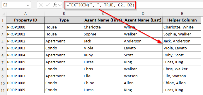
➤ If you have the names in two different columns of the same row, use this formula to join them with a comma:

➤ Here, C2 and D2 are the cells containing the names. Replace them as needed. Use ranges like A2:D2 to join multiple cells.
➤ Click Enter and drag the formula down to join names in the consecutive cells.

For the Same Column and Different Rows

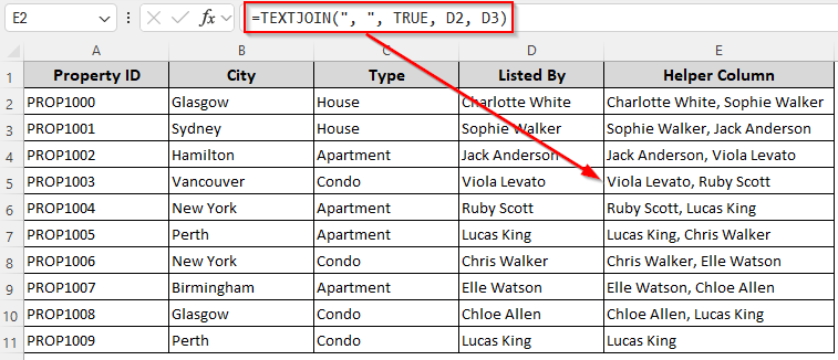
To join the names from the cells of the same column, use this formula:

➤ Replace the cell references D2 and D3 for your source data. Use ranges like D2:D10 for multiple cells.
➤ Click Enter and drag the formula down if required.

Another way of adding a comma between names from two different cells is to use the CONCATENATE (or CONCAT for new Excel versions) function. It combines text from multiple cells into a single cell. Here’s how to use it:

➤ In a helper column cell, enter any of the following formulas:

For the Same Row and Different Columns

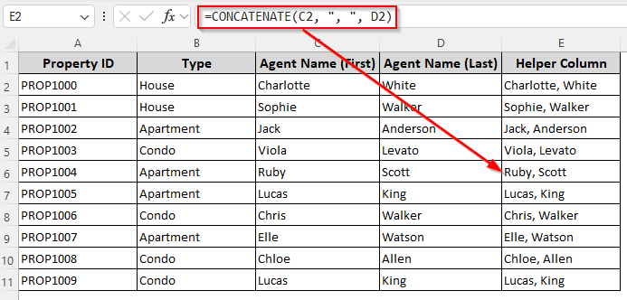
➤ Use this formula to add names from different columns:

➤ Change the cell references C2 and D2 according to your dataset.
➤ Press Enter and drag the formula down to autofill the remaining cells.

For the Same Column and Different Rows

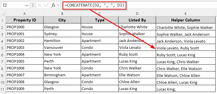
➤ Add names from two different rows and the same column with this formula:

➤ Replace the cell references D2 and D3 with your original source data.
➤ Press Enter and drag the formula down with the fill handle.

With the Power Query tool, you can merge names from different cells with a comma between them. It’s a reliable method for large datasets with multiple columns to merge. For this, follow the steps given below:

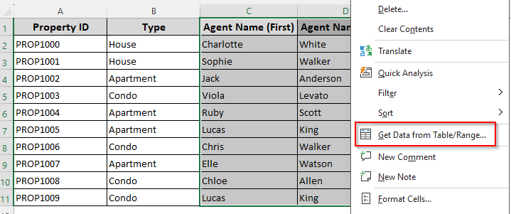
➤ Select the range with the names you want to merge and right-click on your selection. Choose Get Data from Table/Range.

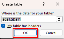
➤ As Excel prompts to turn your data range into a table, press Ok.

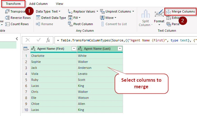
➤ In the Power Query Editor, press the  CTRL  key and select all the columns containing the names.
➤ Now, go to the Transform tab and select the Merge Columns option.

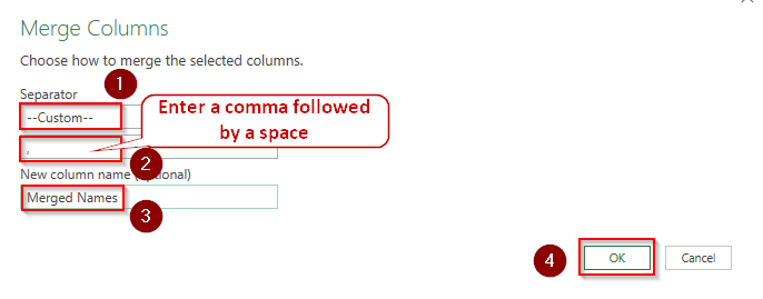
➤ In the Merge Columns dialog box, click on the Separator drop-down and choose Custom. Type a comma and a space in the blank field.
➤ Add a name for the new column with the merged names and click Ok.

➤ As the names are now separated by commas, go to the File tab and click on the Close & Load drop-down and choose Close & Load To.

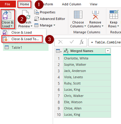
➤ Select a location to put the new column and click Ok. Here’s the final result for our dataset:

In this method, we’ll create a custom VBA code that can add a comma between the names of the same cell or different cells. Let’s get straight to the steps:

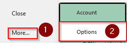
➤ If you don’t have the Developer tab in your main ribbon, go to the File tab >> More >> Options.

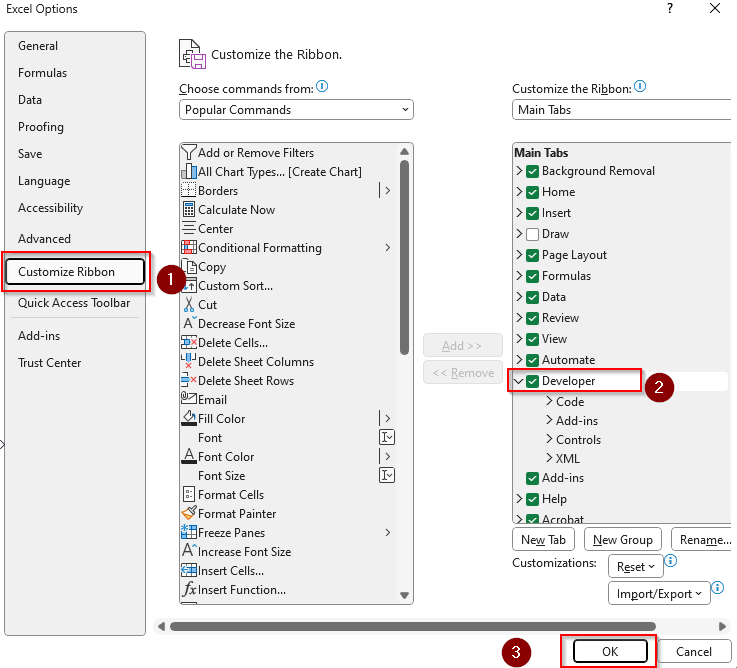
➤ Choose the Customize Ribbon option and check the Developer box. Press Ok.

➤ Now, click on the Developer tab from the main ribbon and select Visual Basic from the Code group.

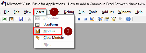
➤ Click on Insert and choose Module from the drop-down menu.

➤ In the blank module field, paste the following code:

Sub CombineNamesUnified()
    Dim userChoice As Variant
    userChoice = MsgBox("Do you want to combine names from the SAME cell?" & vbNewLine & _
                        "Click 'No' to combine names across MULTIPLE columns (row by row).", _
                        vbYesNoCancel + vbQuestion, "Choose Method")
    If userChoice = vbCancel Then Exit Sub
    ' Ask for delimiter
    Dim delimiter As String
    delimiter = InputBox("Enter a delimiter (e.g., , or , and space):", "Delimiter", ", ")
    If delimiter = "" Then Exit Sub
    If userChoice = vbYes Then
        ' ===== SAME CELL LOGIC =====
        Dim cellRange As Range
        On Error Resume Next
        Set cellRange = Application.InputBox("Select the cell(s) with names to split and rejoin:", _
                                             "Select Cells", Type:=8)
        On Error GoTo 0
        If cellRange Is Nothing Then Exit Sub
        Dim c As Range
        For Each c In cellRange
            If Trim(c.Value) <> "" Then
                Dim words() As String
                words = Split(Application.WorksheetFunction.Trim(c.Value), " ")
                c.Value = Join(words, delimiter)
            End If
        Next c
        MsgBox "Same-cell names combined with delimiter.", vbInformation
    ElseIf userChoice = vbNo Then
        ' ===== MULTIPLE CELLS (ROW BY ROW) LOGIC =====
        Dim inputRange As Range, outputStart As Range
        Dim r As Long, col As Long, result As String
        ' Select range of names to combine (e.g., A1:B10)
        On Error Resume Next
        Set inputRange = Application.InputBox("Select the range with names to combine row-by-row:", _
                                              "Select Input Range", Type:=8)
        On Error GoTo 0
        If inputRange Is Nothing Then Exit Sub
        ' Select where to start placing results (e.g., C1)
        On Error Resume Next
        Set outputStart = Application.InputBox("Select the first output cell (e.g., C1):", _
                                               "Select Output Start Cell", Type:=8)
        On Error GoTo 0
        If outputStart Is Nothing Then Exit Sub
        ' Loop through each row in inputRange
        For r = 1 To inputRange.Rows.Count
            result = ""
            For col = 1 To inputRange.Columns.Count
                If Trim(inputRange.Cells(r, col).Value) <> "" Then
                    result = result & Trim(inputRange.Cells(r, col).Value) & delimiter
                End If
            Next col
            ' Remove last delimiter
            If Right(result, Len(delimiter)) = delimiter Then
                result = Left(result, Len(result) - Len(delimiter))
            End If
            ' Output in corresponding row
            outputStart.Cells(r, 1).Value = result
        Next r
        MsgBox "Names from different columns combined row-by-row.", vbInformation
    End If
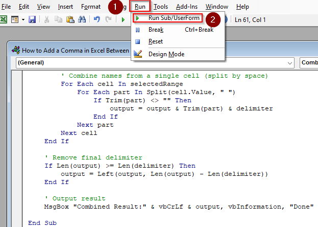
End Sub

➤ Press  F5  or click on the Run tab >> Run Sub/UserForm.

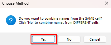
➤ Select whether you want to add a comma between the names of the same cell or different cells. Press Yes for names in the same cell or press No for names in different cells.

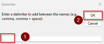
➤ Type a delimiter to add between the names. You can use just a comma or a comma followed by a space for more accuracy. Press Ok.

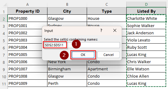
➤ As Excel prompts you to select the cells, go back to the Excel tab and highlight the cells with names. Click Ok.

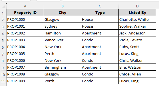
➤ The final result should look like this:

Frequently Asked Questions

How to flip the first & last names and add a comma between them in Excel?

For first and last names that are separated by a space, use this formula in a helper column cell:
=RIGHT(D2,LEN(A1)-FIND(” “,D2)) & “, ” & LEFT(A1,FIND(” “,D2)-1)
Replace D2 with your source cell reference containing the first and last name. Press Enter and drag the formula down if needed.

How to add a comma in numbers automatically in Excel?

First, select the cell(s) with your number and right-click on your selection. Choose Format Cells from the toolbar. Click on the Number tab, select Number. Check the Use 1000 Separator (,) box and click OK. This will format 1000 as 1,000 automatically.

How do you add a symbol between text in Excel?

If your first text is in cell C2 and the second one in cell D2, use this formula to add a dash(-) symbol between them:
=C2 & “-” & D2
You can replace “–” with any symbol you want (e.g. @,*, #).

How do I add text between numbers in Excel?

Let’s say the first number is in cell C2 and the second one is in cell D2. To add a specific text like USD between these numbers, insert the following formula in a helper column cell:
=CONCATENATE(C2, “USD”, D2)
Press Enter and drag the formula down to the remaining cells using the fill handle.

Concluding Words

While choosing a method, consider how large is your dataset and whether the names are in the same or different cell. Methods like using the Flash Fill feature and Find & Replace tool are quick and easy solutions for small datasets. However, automating the process with a formula, Power Query tool, or VBA coding is better for larger datasets as they offer more accuracy.