
When we add, change, or remove any data in Excel, we often need to update formulas, charts, or other related calculations manually, which can lead to mistakes. In such cases, creating a dynamic range allows these elements to update automatically whenever the original data changes. This not only improves accuracy but also saves time. For creating such a dynamic range, the OFFSET function is one of the best choices as it offers flexibility in defining ranges.
In this article, we will explain how you can create dynamic ranges using the OFFSET function in Excel.
➤ First, select cell F1 and write down a name.
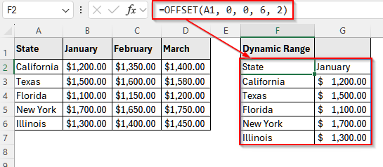
➤ Then, select cell F2 and insert the following formula:
=OFFSET(A1, 0, 0, 6, 2).
Here, A1 is the starting cell reference from where the offset function will count the row and column, the first 0 is the number of rows from the starting cell, the second 0 is the number of columns from the row, 6 is the height of the range and 2 is the width.
➤ Now, press Enter and the dynamic range will be created.
Create a Simple Dynamic Range Using the OFFSET Function in Excel
While the OFFSET function in Excel is flexible and can be used in conjunction with various other functions, it can also create dynamic ranges independently. This function has 5 attributes. One reference cell or starting cell, followed by the distance of the starting row from the starting cell in number, the distance of the starting column from the cell reference in number, the height of the dynamic range, and the width of the dynamic range.
The syntax of the OFFSET function is: =OFFSET(reference, rows, cols, height, width).
We will use the dataset below to explain this formula clearly to you. Let’s take a look.
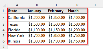
It is sales data of a store across five states of the US. We will create a dynamic range for January month sales across the states.
Steps:
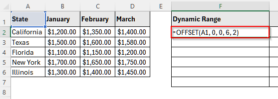
➤ First, select cell F1 and write Dynamic Range.
➤ Now, select cell F2 and insert the following formula:
=OFFSET(A1, 0, 0, 6, 2)
Here, A1 is the starting cell reference from where the offset function will count the row and column, the first 0 is the number of rows from the starting cell, the second 0 is the number of columns from the row, 6 is the height of the range and 2 is the width.
➤ Now, press Enter, and you will see the OFFSET function return the dynamic range for the January month sales data for all states.
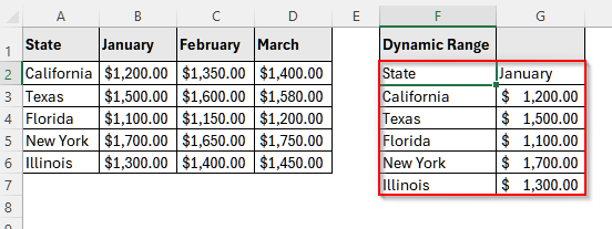
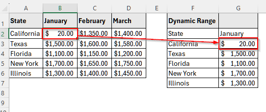
➤ Finally, to check whether the formula automatically updates any changes inside the range, we will change the sales value for California from $1,200.00 to only $20.00. And, you will see that the OFFSET function will update it automatically.
Create Dynamic Range With OFFSET and COUNTA Function in Excel
The COUNTA function can automatically count non-empty cells in a range and if used with the OFFSET function, it can automatically update the dynamic range in case new data is added. Such as, if we create a dynamic range for January month and add a new state to the dataset, it will automatically update the range.
Let’s take a look at how it works.
Steps:
➤ First, select cell F1 and write a suitable name.
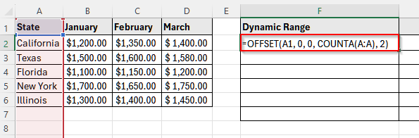
➤ Then, click on cell F2 and insert the following formula:
=OFFSET(A1, 0, 0, COUNTA(A:A), 2)
Here, A1 is the starting cell, the first 0 is the number of rows from the starting cell, the second 0 is the number of columns from the row, COUNTA(A: A) counts the non-empty cells in column A, and the last 2 represents the width.
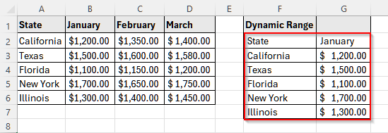
➤ Press Enter and it will return the sales data for January month across all the states.
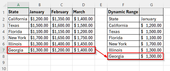
➤ Now, we will add another row in the original dataset for Georgia and the dynamic range will update itself automatically to show the new entry.
Frequently Asked Questions
Can I Use the OFFSET Function with the Sum Function in Excel?
Yes, you can use the OFFSET function with the SUM function in Excel. It will automatically update the sum if you change the values inside the dynamic range. Suppose, you have data from B2 to B5 cells and you want to make a dynamic range and sum the values inside the range. Then, insert the following function into any empty cell:
=SUM(OFFSET(B2, 0, 0, 5, 1)). Now, if you update a value inside this range, such as changing the value of the B3 cell, it will update the sum automatically.
Can I Use the INDEX Function Instead of the OFFSET Function to Make a Dynamic Range in Excel?
You can. However, there is a small difference between these two functions. While both are great for creating dynamic ranges, the OFFSET function is volatile, i.e., recalculates every time. On the contrary, the INDEX function is non-volatile. It only recalculates if data inside the dynamic range changes. Thus, the INDEX function is faster than the OFFSET function in the case of a large dataset.
Why Do I Keep Getting #REF Error After Using the OFFSET Function?
If the range you trying to use is invalid, you will get the #REF error after using the OFFSET function. Such as, if you remove the first cell reference, or use a negative value in width or height, you will get a #REF error.
Wrapping Up
In this article, we have learned to use the OFFSET function in Excel to create a dynamic range both by itself and with the COUNTA function. The OFFSET function is flexible and can accommodate other functions too. Try these methods and share your experience with us.