
Copying formulas in Google Sheets is a simple task essential for data management. However, when users copy formulas to a new location, Google Sheets automatically updates the cell references relative to their new position. While this functionality is often helpful, it can cause errors when the original cell references need to be preserved. There are multiple methods that we can follow to solve this issue in Google Sheets.
To copy formulas and preserve cell references in Google Sheets, follow the steps below:
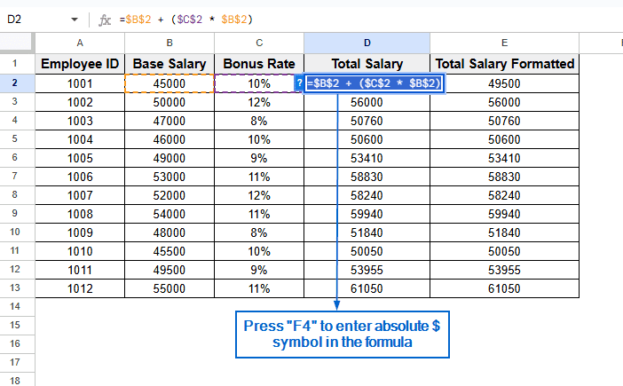
➤ Select the cell with the formula whose cell reference you want to preserve.
➤ Double click on that cell, highlight the formula and add an absolute sign ($) by pressing the F4 key on your keyboard.
➤ Now you can copy and paste the formula anywhere you want, with a locked cell reference.
In this article, we will learn four effective methods for copying formulas in Google Sheets without changing the cell reference.
Copy Formula Using Absolute Cell References
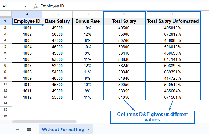
Absolute references, often denoted by the $ symbol, help lock a formula’s cell reference. This method prevents the formula from changing when copied to another cell. In the sample dataset, we have information about Employee ID, Base Salary, Bonus Rate and Total Salary in columns A, B, C, and D, respectively. As we can see in the “Without Formatting” worksheet, copying data from column D (Total Salary) to column E (Total Salary Unformatted) gives us an incorrect value because the formula references shift during the copy.
By using Absolute references, we will copy all formulas and contents from column D to column E while maintaining the original cell references. The results will be displayed in a new worksheet called “ Using Absolute Reference” where Column E displays the total Salary of the employees, formatted to maintain consistent references during copying.
Steps:
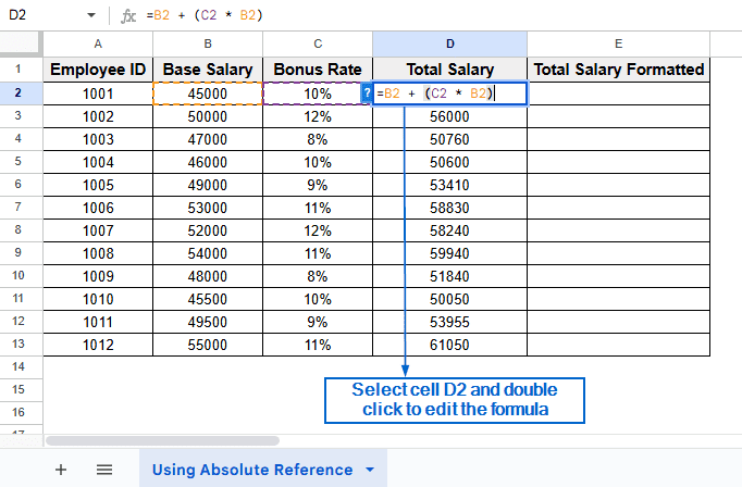
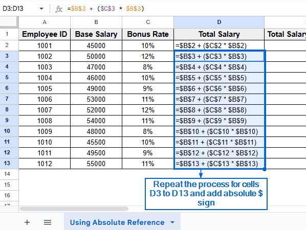
➤ In the “Using Absolute Reference” worksheet, select cell D2 and double-click on it. You should now be able to edit the formula.
➤ Next, highlight the entire formula and press F4 on your keyboard. This action locks in the cell reference by adding an absolute $ sign.
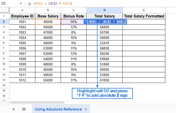
➤ Now repeat the process for cells D3 to D13.
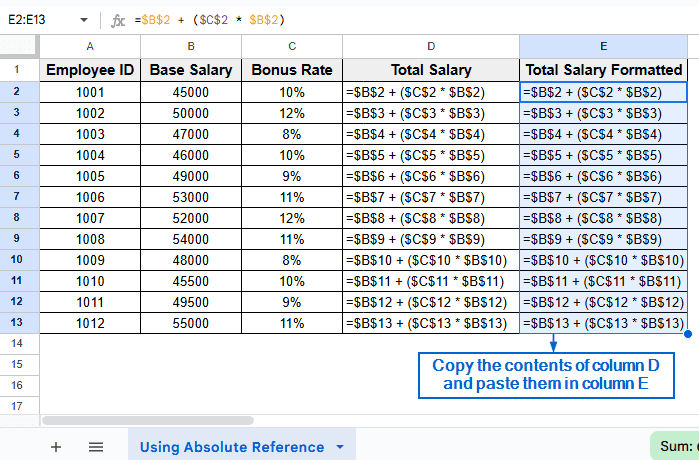
➤ After successfully adding a dollar($) sign to all cells (D2 to D13), simply copy all contents from column D and paste it in column E.
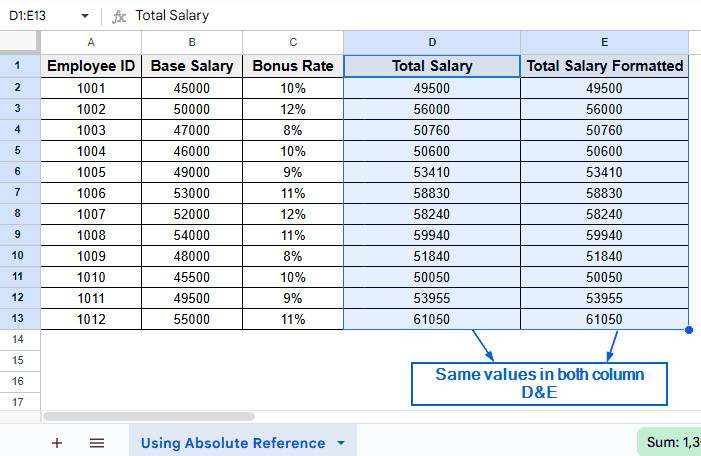
➤ You should now have the same values in column D and column E.
Copy Formula Using Find and Replace Tool
This is a clever and simple method for copying formulas without changing the cell references. This technique uses Google Sheets’ Find and replace tool to temporarily convert a formula to text, allowing users to copy it in other cells, preserving cell references. We will work with the same dataset and display the result in “Using Find and Replace Tool” worksheet.
Steps:
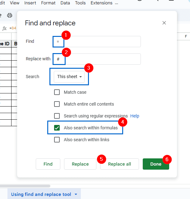
➤ Head to “Using Find and Replace Tool” worksheet and press Ctrl + H to bring out the Find and replace menu.
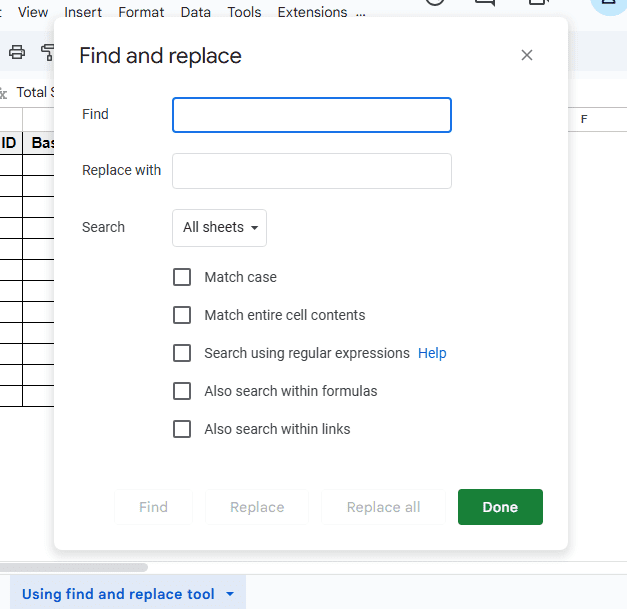
➤ In the Find and replace menu,
➧Type “=” in the Find box.
➧Type “#” in the Replace with box.
Make sure to set the search parameter within “This sheet” and check the “Also search within formulas” box. Then, press the Replace all >> Done button.
Note:
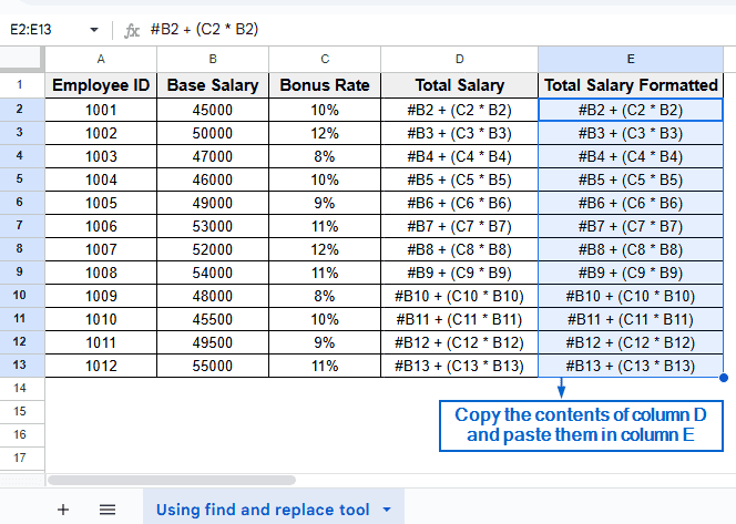
This method converts all formulas into plain text by adding a # symbol in front of them. It will allow us to copy and paste the formulas into our desired cell.
➤ Then, copy the modified plain text versions of the formulas from column D and paste them into column E.
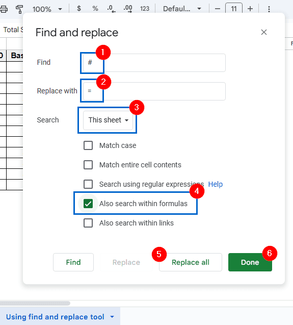
➤ Next, press Ctrl + H again and bring out the Find and replace menu. This time,
➧Type “#” in the Find box.
➧Type “=” in the Replace with box
Again, set the search parameter within “This sheet” and check “Also search within formulas” box. Then, click on Replace all >> Done to complete the operation.
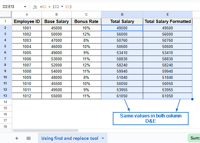
➤ You should now see both column D and column E showing the same results, each containing the same formulas.
Copy Formula Using Plain Text Method
The Plain text method is another effective way of copying formulas in Google Sheets without changing the cell references. For this technique, we need to use Notepad or any other plain text editor. We will again work with the same dataset and, using the Plain text method, copy formulas from column D to column E without changing the cell reference. The results will be displayed in “Using Plain Text Method” worksheet.
Steps:
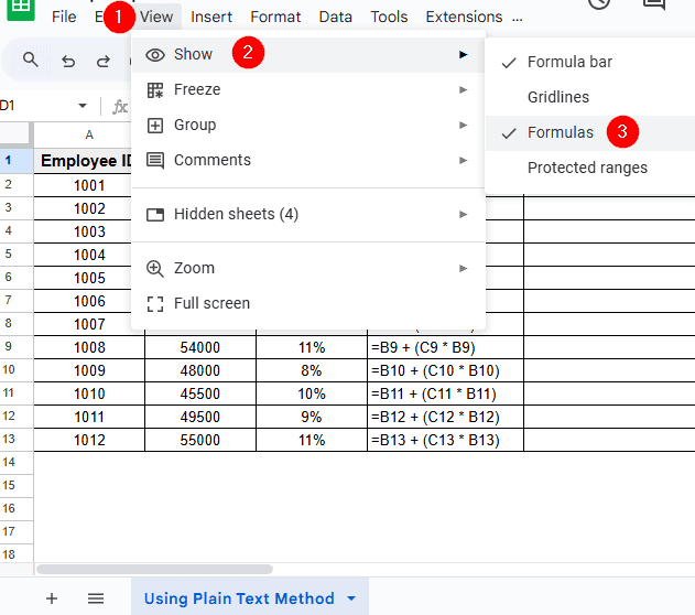
➤ Open the “Using Plain Text Method” worksheet. From the main menu, head to View >> Show and check the Formulas option. The formulas used in column D should be visible now.
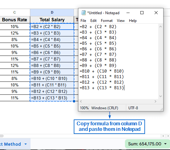
➤ Next, open a text editor of your choice. In our case, we will use Notepad. Copy the formulas from column D and paste them into Notepad.
Note:
This method converts the formulas in column D into plain text, allowing us to paste them in column E without altering cell references.
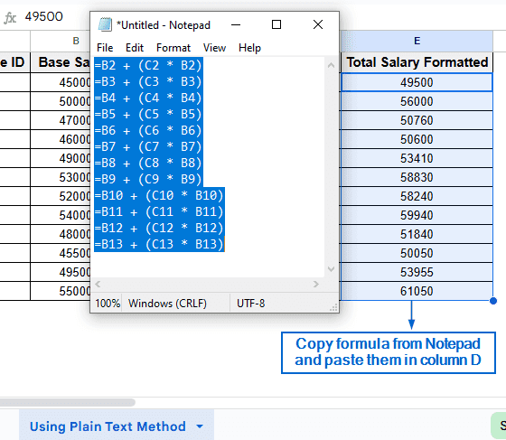
➤ Now, copy the formulas from Notepad and paste them in column E. It should automatically display the same data as column D.
➤ Lastly, head to View >> Show and uncheck the Formulas option from the main menu to complete the operation.

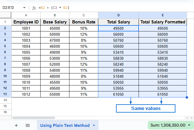
➤ Both columns C & D should now display the same result.
Copy Formula Using ARRAYFORMULA Function
This is the quickest and most efficient method for copying formulas while preserving cell references. ARRAYFORMULA in Google Sheets is a powerful function that lets users apply a formula to an entire range of cells at once, saving time and improving efficiency. Unlike other methods, you don’t need to follow lengthy procedures for keeping cell references unchanged. We will use the same dataset used in other methods, and this time use ARRAYFORMULA to copy the contents from column D to column E. We will display the result in “Using Arrayformula” worksheet.
Steps:
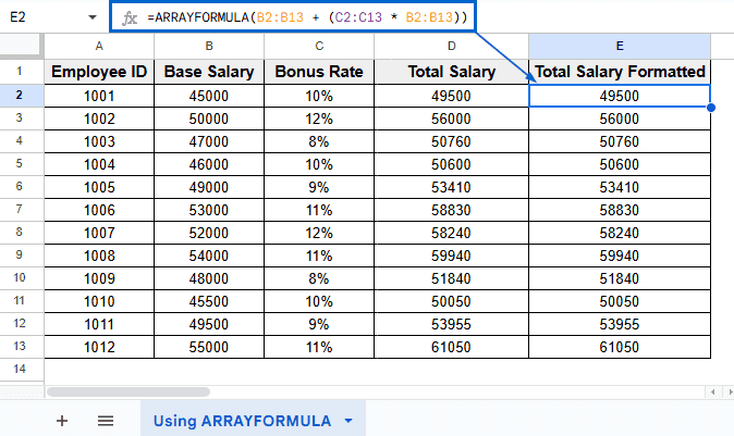
➤ Open “Using ARRAYFORMULA” worksheet and in cell E2 put the formula:
=ARRAYFORMULA(B2:B13 + (C2:C13 * B2:B13))
Note:
In the formula, B2:B13 and C2:C13 refer to the Base Salary and Bonus Rate columns, respectively. (C2:C13 * B2:B13) part of the formula is used to calculate the bonus amount of each employee, and (B2:B13 + (C2:C13 * B2:B13) adds the base salary to the bonus amount to get the total salary. Finally, ARRAYFORMULA is used to run the formula across all rows all at once.
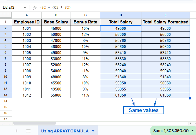
➤ Press Enter. You should now see that all the information from column D has been automatically transferred to column E with the cell references and formulas preserved.
Frequently Asked Questions
How do I Know If My Copied Formulas are Producing Correct Results?
By comparing the values in the target column with the original column, you can easily find out whether your copied formulas are producing correct results or not. If the values of both columns match, you will know that the formulas were copied correctly with preserved references.
Which Method Should I Use For Large Datasets?
If you are working with large datasets, then the ARRAYFORMULA method will be the best option for you. Since you only need to write the formula once, there is no need to copy it manually.
Concluding Words
Copying formulas without changing cell references is crucial for maintaining accuracy in Google Sheets. In this article, we have discussed four important methods for copying formulas without changing cell references, including using Absolute references, Find and replace tool, Plain text and the ARRAYFORMULA function. Feel free to experiment with each method to find out the one that best aligns with your needs.