While dealing with numbers in Google Sheets, sometimes we need to round numbers quite a bit, not just to whole numbers, but to the nearest 5, 10, 100 or an another order. Whether it’s pricing adjustments, scheduling tasks, or stock management in steps of five, rounding to the nearest 5 can make your data neater and even more practical.
For example, you may have a list of times and you’d like to round them to the nearest 5 minutes to make them align or be more tasteful in a schedule. Or you want to make sure your sales price always ends in.00 or.50. These are all instances where rounding to the nearest 5 makes things clearer and more consistent.
➤ Select the cell where you want the rounded number to go.
➤ Enter the formula: =MROUND(C2, 5), where C2 stands in for the cell you’re referencing.
➤ Press Enter and the value in cell C2 is now rounded to the nearest 5.

This technique involves Google Sheets’ MROUND function, which rounds numbers to a multiple you specify 5, in this case. In this tutorial, I’m going to show you how to round numbers to the nearest 5 in Google Sheets. I will also give you a few suggestions to solve common problems while using the counter with negative numbers or decimals.
How Rounding Works: Why Nearest 5?
If we round a number to the nearest 5, we change it to the nearest multiple of 5. In other words, we want to round down by 5, or in practical terms, we should look for the closest number divisible by 5: 0, 5, 10, 15, 20, so on and so forth.
To find the nearest multiple of 5:
➤ If it’s halfway between two multiples of 5, round up to the bigger one.
➤ Otherwise, we round to the closest multiple of 5.
Examples:
➤ 12 is closer to 10 than it is to 15, hence, it gets rounded up to 10.
➤ 13 is closer to 15, so it rounds up to 15.
This formula acts as a way of simplifying numbers, while also keeping them as accurate and useful as they can be. However, there are generally three kinds of rounding to think about:
➤ ROUND: Rounding to the nearest. It uses the rounded value to the nearest multiple given by here.
➤ ROUNDUP: Round up (ceiling) always rounds up to next multiple.
➤ ROUNDDOWN: Rounding down (floor) rounds down to the nearest previous multiple.
Or, depending on your purpose, you can also use a different rounding approach.
Now that we know how rounding works, let’s discuss how to round to the nearest 5 in Google Sheets. There are typically five different functions you can choose from while rounding nearest. Among them, the first and the best one would be the MROUND function. So, let’s begin with that.
Round to the Nearest 5 with MROUND Function
The MROUND function in Google Sheets returns a number rounded to the nearest multiple of a number that is given. And unlike ROUNDUP or ROUNDDOWN that always round in one direction (up or down), MROUND will select the nearest multiple, up only if the number is closer to the larger multiple. It’s especially helpful for rounding to the intervals, like 5, 10, or 0.25.
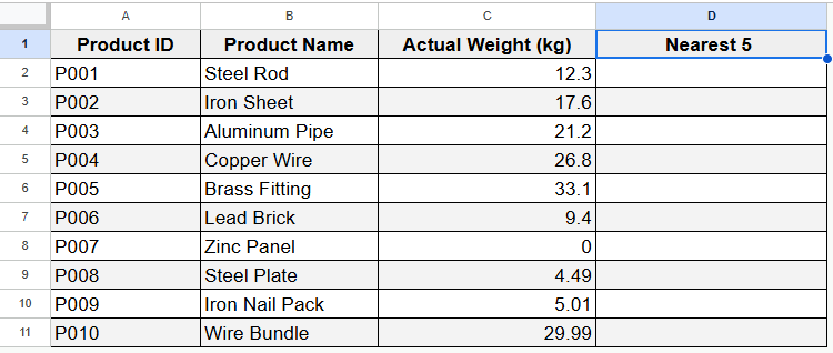
In the following dataset, there are some numeric values in column C including decimal points. In column D, we’re going to round all the values present in column C to the nearest 5.
Steps:
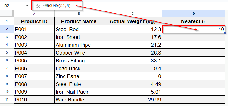
➤ Select the output cell D2 and type the following formula:
=MROUND(C2, 5)
➤ Press Enter and you’ll see the number 12.3 is rounded to 10 in the output cell D2.
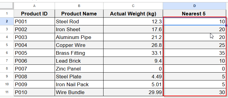
➤ Now use the FIll Handle to drag the D2 down to the D11 and you’ll find all other cells with the rounded values of the corresponding decimal values present in Column C.
Round To the Nearest 5 With ROUNDUP Function
The ROUNDUP function rounds a number away from 0, regardless of the value of the next digit. On the other hand, the ROUND function rounds off depending on rounding rules and ROUNDDOWN always rounds down towards zero. This is where ROUNDUP comes in handy when you just need a higher result like when you need to calculate for number of resources or packaging.
Steps:
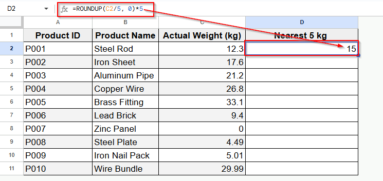
➤ Click cell D2 as we’re using it to be the active cell.
➤ Now type the formula as follows:
=ROUNDUP(C2/5, 0)*5
➤ Press Enter and the result will be 15 which is the next number that is a multiple of 5 after 12.
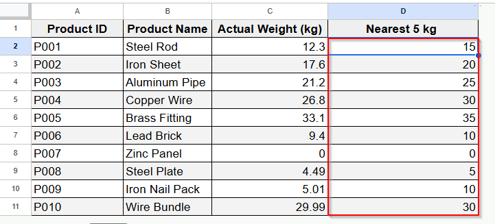
➤ Then simply drag the Fill Handle down to the D11 cell or click the Auto Fill tick mark to get the rounded values automatically to the other cells of the D column.
Round to the Nearest 5 with ROUNDDOWN Function
The ROUNDDOWN function in Google sheets always rounds a number down toward zero, no matter what digit comes after the rounding place. Unlike ROUND, which follows standard rounding rules, and ROUNDUP, which always rounds up, ROUNDDOWN ensures the result is never greater than the original number. It’s useful when you want to stay within a limit or avoid exceeding a value.
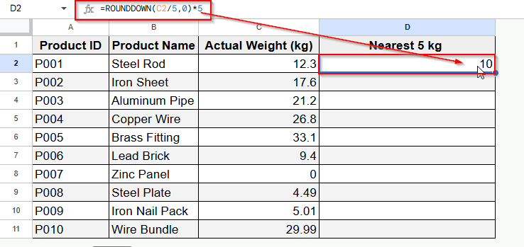
➤ Just as the previous two methods, click cell D2 to make it the active cell.
➤ Now insert the formula =ROUNDDOWN(C2/5, 0)*5 inside the cell.
➤ Press Enter and the result is 10, the next number below 12.3 that is a multiple of 5.
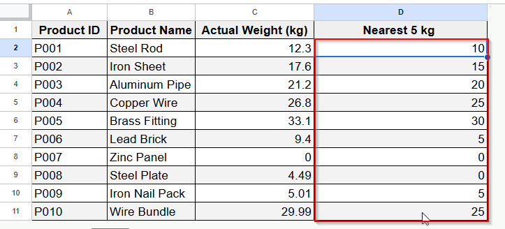
➤ Finally drag the FIll Handle from the D2 cell to the D11 and all other cells will be filled with the rounded values of the cells in Column C.
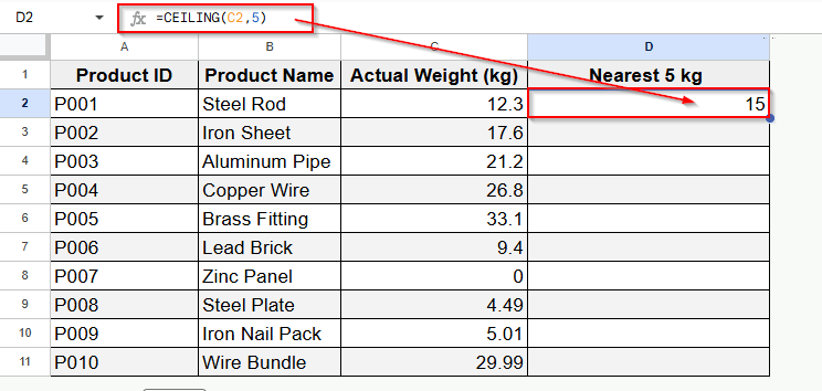
Round Up to the Nearest 5 with CEILING Function
The CEILING function in Google Sheets rounds a number up to the nearest multiple of a specified value. Unlike standard rounding, which rounds to the nearest value, up or down, the ceiling function always rounds upward, regardless of the decimal. For example, CEILING(12.3, 5) returns 15, while ROUND(12.3, -1) would return 10.
Steps:
➤ Tap on an active cell just like we’re using D2 cell here.
➤ Next, enter the formula shown below:
=CEILING(C2, 5)
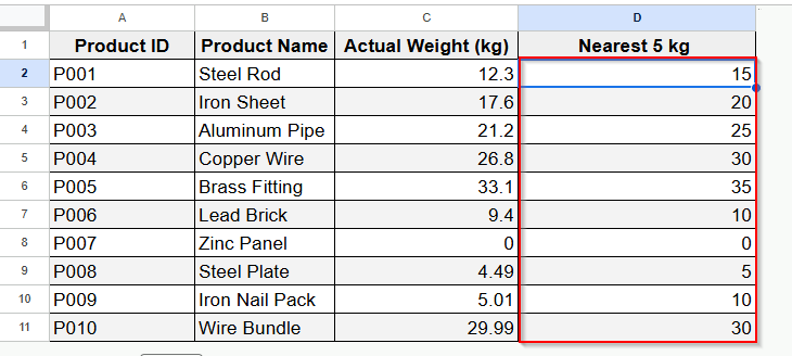
➤ Press Enter and the result will be 15.
➤ Now just drag the Fill Handle down to cell D11 or click the Auto Fill tick mark to automatically fill the rest of the D column with the rounded values.
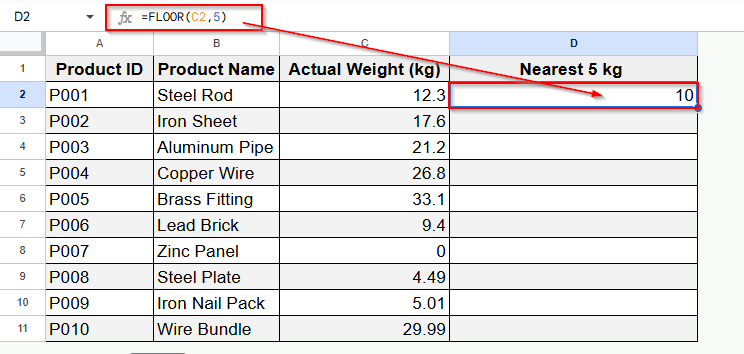
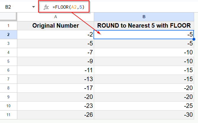
Round Down to the Nearest 5 with FLOOR Function
The FLOOR function in Google Sheets rounds a number down to the nearest multiple of a specified value. Unlike standard rounding, which goes to the closest value, or the CEILING function, which always rounds up, FLOOR always rounds downward. For example, FLOOR(12.3, 5) returns 10, while ROUND(12.3, -1) would round to 10, but CEILING(12.3, 5) would return 15.
Steps:
➤ Click on cell D2.
➤ Then type formula =FLOOR(C2, 5) and press Enter. Here, the result will be 10 as we can see in the image below.
➤ Now drag the Fill Handle from D2 down to D11, and you’ll see all the cells filled with rounded values matching the decimal numbers in Column C.
Rounding Negative Numbers to the Nearest 5
First of all, MROUND works on negative numbers in the usual manner, that is rounding to the closest multiple.
This means that using MROUND(-13, 5) will return -15, because -15 is closer to -13 than -10. No matter whether the number is positively or negatively rounded, it will always be rounded towards the closest multiple.
Therefore, unlike CEILING and FLOOR funtcions, MROUND takes what’s nearest, which clearly shifts the rounding process in a more balanced direction.
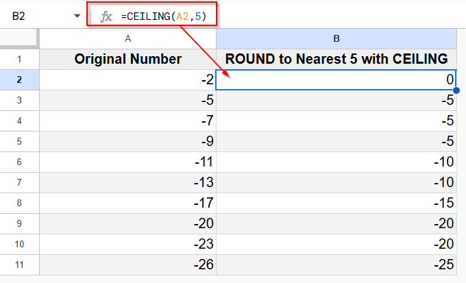
But CEILING and FLOOR are different.
➤ For positive numbers, they behave just as expected (up or down).
➤ For negative numbers, CEILING rounds toward zero, and FLOOR rounds away from zero.
For example: CEILING(-2, 5) = -0 while FLOOR(-2, 5) = -5. This could be useful depending on whether you need to maximize or minimize the absolute value of a negative number.
Additionally, this distinction is important in scenarios like scheduling or inventory where rounding direction affects outcomes. For instance, CEILING can help round negative durations or stock deficits toward zero to avoid overestimation, while FLOOR can be used to ensure conservative estimates or buffer zones by rounding further away. Following is an example of what the CEILING function does to the negative numbers.
And below is another output with the FLOOR function applied to the negative numbers. It’s simply rounding the negative numbers away from 0..
These equations are simple to use and may save you time on reports and in calculations. Need to round to the nearest 5, 10, 100 etc? Just change the second argument in the formula.
Tips and Troubleshooting While Rounding Numbers
- Negative numbers: MROUND() also handles negative numbers. For instance, =MROUND(-12, 5) will round down to -10.
- Zero and non-numeric inputs: Make sure your cells actually have numbers in them, otherwise MROUND() will throw an error.
- Decimals: If you want to round to the nearest 0.05 then just adjust the multiple argument: =MROUND(1.23, 0.05) will round to 1.25.
- Big sheets: If you are working with large datasets, MROUND() helps keep your formulas short and fast instead of long, complex and dirty nested formulas.
Frequently Asked Questions (FAQ)
Can I round to the nearest 5 without using MROUND()?
Yes, but with less efficiency. You would then divide by 5, round and multiply back like =ROUND(A1/5)*5. MROUND() is simpler.
Is there a function that will round a value up to the nearest multiple of 5?
You can use CEILING, for example: =CEILING(A1, 5).
Can time amounts be rounded to the nearest 5 minutes?
Yes, use =MROUND(A1, TIME(0,5,0)) instead – as time is in fractional days in Sheet.
Concluding Words
If you use Google Sheets and you want to round to the nearest 5, it’s easy to do once you know how. With the MROUND function, you can round any number to your preferred multiple, so your data remains clean and helpful. Whether you need to deal with prices, schedules or quantities, this small formula can help automate, systemize, and accelerate tasks you do on the spreadsheet.
Next time you come across such data that you need to figure out how to round to the nearest 5, do not forget that =MROUND(Value, Factor) can help you do it in an easy and clean way.