
When working with datasets in Excel, it is often required to assign values based on ranges, such as determining student grades from scores or employee bonuses from sales figures. Although we can easily find value that falls between a range with the help of VLOOKUP function, there are other methods as well that let users perform this operation efficiently.
Follow the steps below to use VLOOKUP for finding a value that falls between a range:
➤ In your dataset, select the cell where you want to display the found value and put the formula:
=VLOOKUP(lookup_value, table_array, col_index_num, [range_lookup])
➤ Replace “lookup_value” in the formula with the value you want to search.
➤ Replace “table_array” with the range of cells that contains the data you want to search.
➤ Replace “col_index_num” with column number from which to return a result.
➤ Finally, Replace “[range_lookup]” with TRUE for an approximate match and FALSE for an accurate match.
In this article, we will learn how to use VLOOKUP function to find a value that falls between a range. We will also cover three alternative methods to VLOOKUP that allow you to perform this operation more efficiently.
Use VLOOKUP to Return Values Within a Range
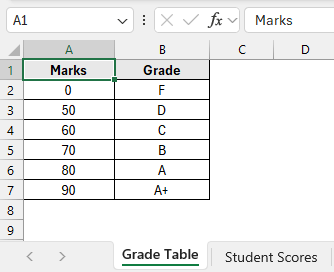
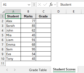
In the sample dataset, we have two separate worksheets. The Grade Table worksheet contains information about Marks and Grades. Meanwhile, the Student Scores worksheet contains information about Student names, Marks and an empty Grade column.
By using the VLOOKUP function, we will return the appropriate grade in column C of the Student Scores worksheet based on each student’s marks, referencing the grading criteria defined in the Grade Table worksheet. We will display the updated dataset in a separate “VLOOKUP Function” worksheet.
VLOOKUP in Excel is a useful function that allows users to search for a specific value in the first column of a range and return a corresponding value from another column within the same range.
Steps:
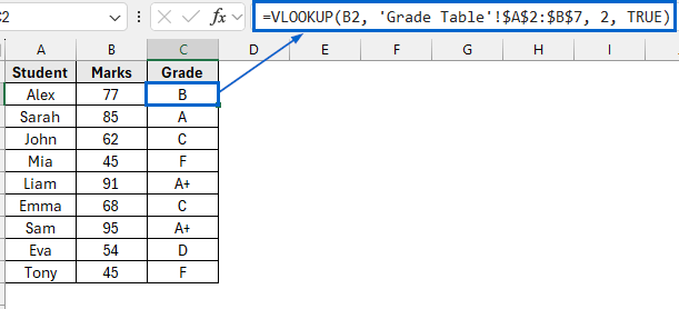
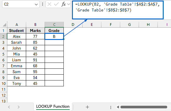
➤ Open the VLOOKUP Function worksheet and in cell C2, put the following formula:
=VLOOKUP(B2, 'Grade Table'!$A$2:$B$7, 2, TRUE)
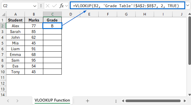
➧ B2 is the lookup value that contains the score for which we want to find the corresponding grade.
➧ Grade Table'!$A$2:$B$7 is the range of cells in columns A and B of the Grade Table where Excel looks for the value.
➧ 2 tells Excel to return the value from the second column of the specified range.
➧ TRUE tells formula to return an approximate match.
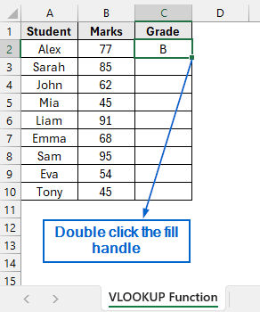
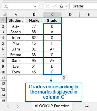
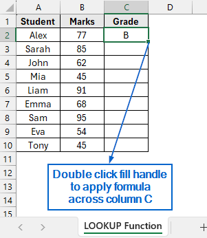
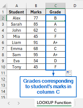
➤ Next, select cell C2 again and double-click the fill handle to apply the formula across column C.
➤ Grades corresponding to the marks obtained by the students should now be visible in column C.
Alternatives to the VLOOKUP Function for Finding Value Falling Between a Range
While the VLOOKUP function is commonly used to find values within ranges, it has its limitations. For instance, VLOOKUP function requires the lookup column to be the first in the range, severely limiting flexibility. Whereas alternatives like LOOKUP, INDEX-MATCH, and CHOOSE–MATCH functions do not have this constraint, offering greater versatility.
Use LOOKUP Function for Simplified Range Matching
In Excel, the LOOKUP function is a straightforward tool used to find a value in a range or array and return a corresponding value from another range. Unlike the VLOOKUP function, the LOOKUP function has a simpler syntax and doesn’t require a column index number, making it more beginner-friendly.
Working with the same dataset, we will find out the grades in column C of the Student Scores worksheet based on the range defined in the Grade Table worksheet. We will display the updated dataset in a separate worksheet called “LOOKUP Function”.
Steps:
➤ Open the LOOKUP Function worksheet and in cell C2, put the following formula:
=LOOKUP(B2, 'Grade Table'!$A$2:$A$7, 'Grade Table'!$B$2:$B$7)
➧ “B2” is the lookup value.
➧ “Grade Table'!$A$2:$A$7” refers to the range of scores that the formula searches through to find the closest match for the value in cell B2.
➧ “Grade Table'!$B$2:$B$7” contains the grade we want to return once the appropriate range is identified.
➤ Now, select cell C2 and apply formula to the remaining cells by double-clicking the fill handle.
➤ Column C should now display the appropriate grade based on the marks obtained by the students.
Combining INDEX and MATCH Functions for More Flexibility
The INDEX function in Excel is used to return the value of a cell at a specified row within a given range. Meanwhile, the MATCH function returns the position of a lookup value within a range.
Combining INDEX and MATCH functions provides greater flexibility for performing lookups, as it allows users to retrieve values from any column, regardless of position. It also enables better error handling when used with the IFERROR function.
We will again work with the same dataset and combine INDEX with MATCH functions to assign grades in column C of the Student Scores worksheet, based on the defined ranges in the Grade Table worksheet. The modified dataset will be displayed in a separate worksheet called “INDEX with MATCH Function”.
Steps:
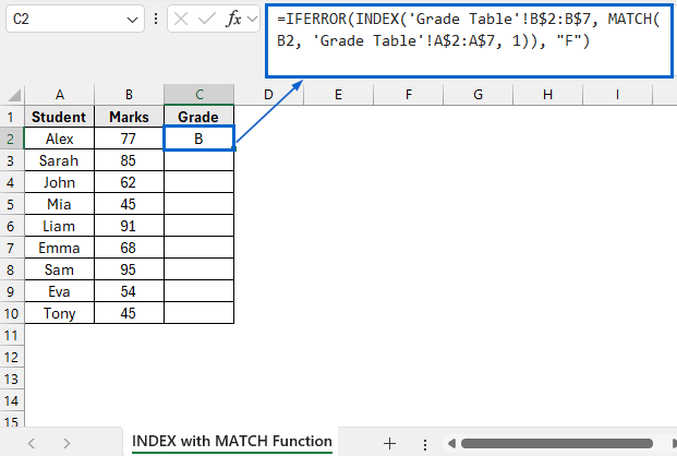
➤ Open the INDEX with MATCH Function worksheet and in cell C2, put the following formula:
=IFERROR(INDEX('Grade Table'!B$2:B$7, MATCH(B2, 'Grade Table'!A$2:A$7, 1)), "F")
➧ MATCH(B2, 'Grade Table'!A$2:A$7, 1) part looks for the largest value in the Marks column that is less than or equal to the value in B2.
➧ INDEX('Grade Table'!B$2:B$7, …) uses the position data from MATCH function to return the correct grade from the Grade column.
➧ IFERROR(…, 'F') acts as a fail-safe, returning grade F if the score in cell B2 is too low to match any value in the range.
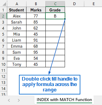
➤ Now, click on cell C2 again and double click the fill handle to apply the formula across the entire range.
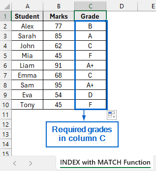
➤ You should now see the corresponding grades for each student’s marks being displayed in column C.
Use CHOOSE with MATCH Functions for Better Customization
This advanced method uses a combination of CHOOSE and MATCH functions to manually create an array for assigning custom ranges. Since CHOOSE and MATCH functions allow you to create and manage custom ranges directly within the formula, you do not need a separate table to define the lookup ranges.
Working again with the same dataset, we’ll determine the grades in column C of the Student Scores worksheet, this time combining CHOOSE and MATCH functions. We will display the modified dataset in a separate worksheet called “CHOOSE and MATCH Function”.
Steps:
➤ Open CHOOSE and MATCH Function worksheet and in cell C2, put the following formula:
=CHOOSE(MATCH(B2, {0,50,60,70,80,90}, 1), "F", "D", "C", "B", "A", "A+")
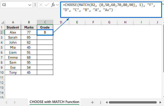
➧ “MATCH(B2, {0,50,60,70,80,90}, 1)” part looks at the number entered in cell B2 and finds out which score range it belongs to.
➧ “CHOOSE(..., "F", "D", "C", "B", "A", "A+")” part uses the number returned by MATCH to pick the corresponding grade from the list.
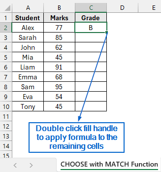
➤ Then, select cell C2 again, double-click the fill handle and apply the formula across column C.
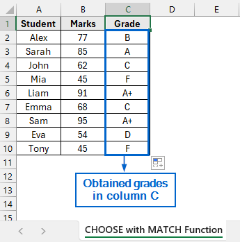
➤ Grades with respect to the marks obtained by the students should now be displayed in column C.
Frequently Asked Questions
Why is VLOOKUP Returning Wrong Result?
VLOOKUP might return a wrong result if the first column of your lookup table is not sorted in ascending order. To avoid this, always ensure that the first column is sorted in ascending order when performing approximate lookups.
Which Lookup Method Should I Use When Dealing With Large Datasets?
For large datasets, the INDEX with MATCH method is generally preferred due to its faster performance, as it targets specific ranges rather than scanning entire columns. It also provides greater flexibility, supporting lookups in any direction.
Concluding Words
Knowing how to use VLOOKUP in Excel to find a value that falls between a range is essential, especially when working with datasets like student grades or commission tiers.
In this article, we have discussed 4 efficient methods on how to use vlookup to find a value that falls between a range, including using VLOOKUP Function, LOOKUP Function, combining INDEX with MATCH function and CHOOSE with MATCH function. Feel free to try out every method and choose one best suited for your needs.