
Combining rows with same ID is often necessary in Excel when dealing with datasets containing multiple entries for the same record, such as transactions, customers, or orders. Although there are no built-in tools in Excel that let users combine rows with the same ID, we can use different functions and formulas to accomplish this task.
Follow the steps below to combine rows with the same ID in Excel:
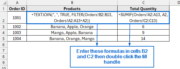
➤ In your dataset, select the cell where you want to display the combined data and paste the following formula:
=TEXTJOIN(“, “, TRUE, FILTER(Orders!B2:B13, Orders!A2:A13=A2))
➤ If you want to calculate the total quantity for the same Order ID, enter the following formula in a separate cell:
=SUMIF(Orders!A2:A13, A2, Orders!C2:C13)
In this article, we will learn 3 effective methods of combining rows with same ID in Excel.
Combine Product Names Using TEXTJOIN and FILTER Functions
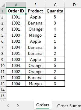
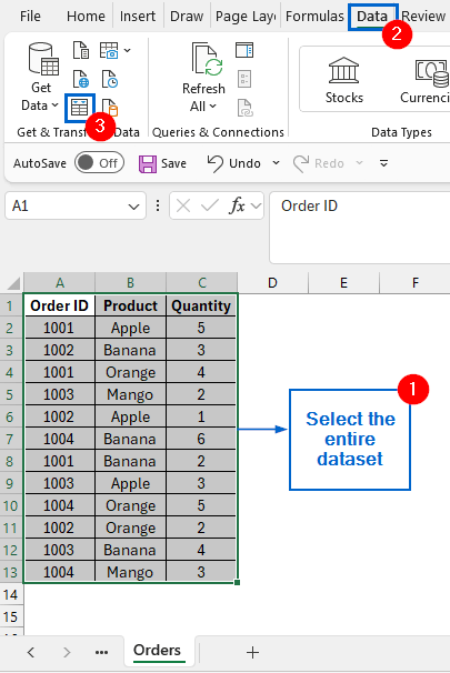
In the sample dataset, we have two separate worksheets called Orders and Order Summary. In the Orders worksheet, we have information about Order ID, Product and Quality.
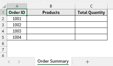
Whereas the Order Summary worksheet contains only the Order ID, along with empty Products and Total Quantity columns.
Using the TEXTJOIN and FILTER functions, we will combine product names based on the corresponding Order ID from the Orders worksheet and display them in column B of the Order Summary worksheet. We’ll also use the SUMIF function to calculate the total quantity of products for each Order ID and show the result in column C of the same worksheet. The updated dataset will be displayed in a separate worksheet called “TEXTJOIN with FILTER Function”.
The TEXTJOIN function in Excel combines text strings from multiple cells or ranges into a single cell. Whereas, the FILTER function retrieves data that meets defined criteria, returning only the rows and columns that match those conditions. Finally, the SUMIF function calculates the total of values in a range that satisfy a given condition, making it useful for conditional summation tasks.
Steps:
➤ Open the TEXTJOIN with FILTER Function worksheet, and in cell B2, put the following formula:
=TEXTJOIN(", ", TRUE, FILTER(Orders!B2:B13, Orders!A2:A13=A2))
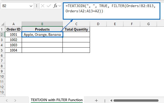
➧ FILTER(Orders!B2:B13, Orders!A2:A13=A2) part extracts all values from the range Orders!B2:B13 where the corresponding value in Orders!A2:A13 matches the value in cell A2.
➧ TEXTJOIN(", ", TRUE, …) part uses the TEXTJOIN function to join all the filtered values into a text string, separating them with commas. The TRUE argument ensures that any empty cells are ignored.
➤ Again, within the same spreadsheet, select cell C2 and paste the following formula:
=SUMIF(Orders!A2:A13, A2, Orders!C2:C13)
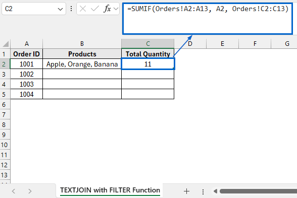
➧ Orders!A2:A13 is the range where Excel looks for matching values.
➧ “A2” is the search criteria, Excel will look for this value in the range.
➧ Orders!C2:C13 is the range of numbers to sum if the corresponding cell in the criteria range matches A2.
➤ Now, double-click the fill handle of cell B2 and C2 to apply the formula across columns B and C, respectively.
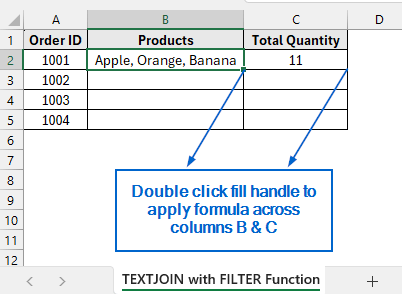
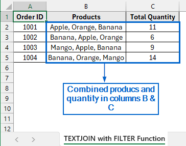
➤ The combined products based on each Order ID, along with their corresponding total quantities, should now be visible in columns B and C.
Combine Rows Automatically Using Power Query
Power Query in Excel is a very powerful tool that enables users to import and transform data according to their needs. This method is particularly effective for combining large datasets, but it can be challenging to set up.
We will work with the same dataset and, using Power Query, combine product names and calculate the total quantity for each corresponding Order ID from the Orders worksheet. The combined product names and the summed quantities will be displayed in columns B and C of the Order Summary worksheet. We will display the updated dataset in a separate “Power Query” worksheet.
Steps:
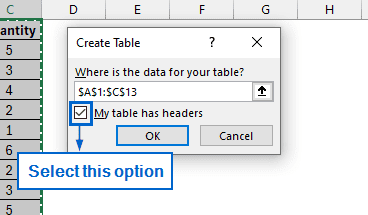
➤ Go to the Orders worksheet, select the entire dataset, and from the Data tab, click on From Table/ Range.
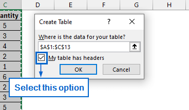
➤ Next, in the Create Table dialogue box, check the My table has headers box.
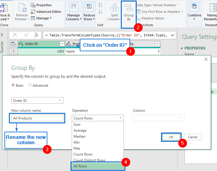
➤ From the Power Query Editor, select Order ID column, then click on Group By.
➤ In the Group By dialogue box, enter All Products as the new column name, and choose All Rows from the operation categories.
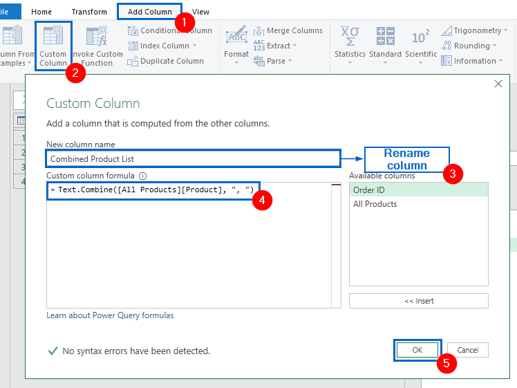
➤ Next, head to the Add Column tab and click on Custom Column.
➤ In the Custom Column dialogue box, type “Combined Product List” under New column name and in Custom column formula, type the following formula:
=Text.Combine([All Products][Product], ", ")
Note:
The formula is used to combine all products in the group with comma as a separator.
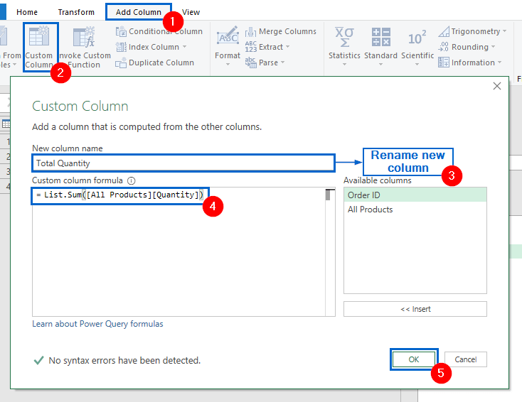
➤ Again, go to the Add Column tab, select Custom Column.
➤ Rename the new column as Total Quantity and in Custom column formula box, enter:
=List.Sum([All Products][Quantity])
Note:
The formula is used to add all quantity values in each group.
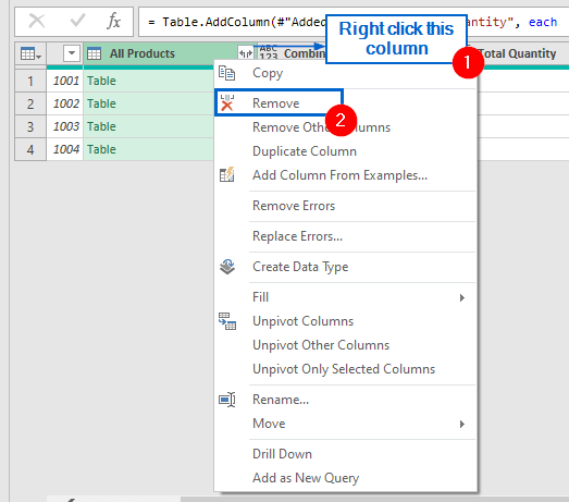
➤ Next, remove the All Products column by right-clicking on it and selecting Remove from the drop-down menu.
➤ Finally, go to the Home tab and click on Close & Load to complete the operation.
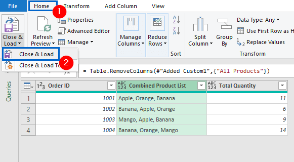
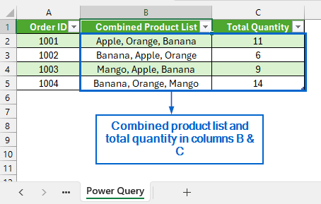
➤ The combined product list, along with the summed quantity, should now be displayed in columns B and C.
Use Pivot Table to Combine Rows by Summing Quantities
The Pivot Table in Excel is used for summarising and presenting large datasets efficiently. Unlike previous methods, this method only allows users to combine rows for calculating the total quantity.
We will again work with the same dataset and use a Pivot Table to summarize the total quantity of products for each Order ID listed in column A of the Orders worksheet. The modified dataset will be displayed in a separate “Pivot Table” worksheet.
Steps:
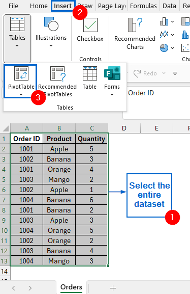
➤ Head to the Orders worksheet and select the entire dataset.
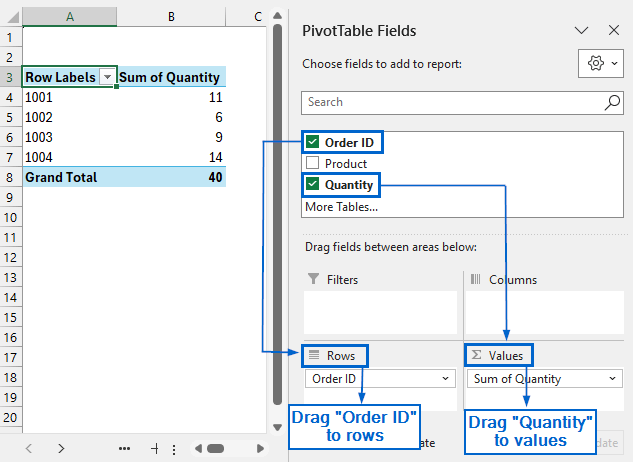
➤ Next, go to the Insert Tab and select Pivot Table.
➤ Check the New Worksheet option in the dialogue box, then click OK.
➤ In the PivotTable Fields pane, drag Order ID to Rows and Quantity to Values.
➤ Rename columns from Row Labels to Order ID and Sum of Quantity to Total Quantity.
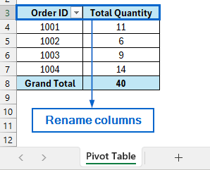
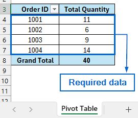
➤ You should now see the total quantities being displayed, grouped by their respective Order ID.
Frequently Asked Questions
Can these Methods be Used for Numerical Data Other Than Quantities?
Yes, you can use all three methods to handle any type of numerical data. For example, the SUMIF function can be used to total any numeric field based on matching IDs or criteria. TEXTJOIN + FILTER can list values like product codes, invoice numbers, or even numeric grades. Power Query and Pivot Table can summarize, group, and aggregate any numeric data.
Why is the FILTER Function Not Working in My Dataset?
The FILTER function is only available in Excel 365 and Excel 2019 or later. If you are using an older version of Excel, this function may not work in your dataset. Consider using array formulas as an alternative, or switch to Power Query for filtering if you are running an older Excel variant.
Concluding Words
Knowing how to combine rows with same ID in Excel is essential for organizing datasets and streamlining workflows. In this article, we have discussed three practical methods of combining rows with same ID, including using TEXTJOIN with FILTER Functions, Power Query and Pivot Table. Feel free to try out each method and choose one that best aligns with your needs.