
When you’re working with lists of names, products, or IDs in Excel, you need to find out which values are common between those values. Manually checking and comparing columns will require a significant amount of time. That’s why Excel has a lot of ways to compare two columns and return only the values that appear in both. In this article, we’ll compare two Excel columns and return common or duplicate values by exploring different methods, including functions, formulas, and conditional formatting rules.
To compare two columns and return common values using the IF and the COUNTIF function, follow the steps below:
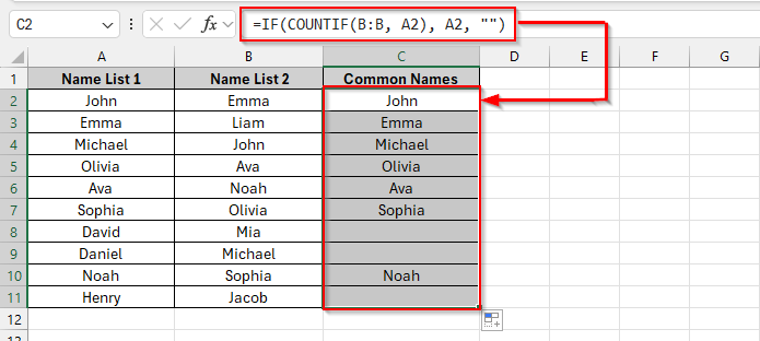
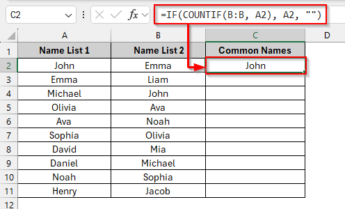
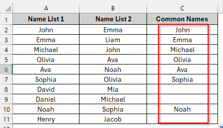
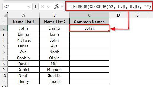
➤ Select the cell on C2 and write this formula: =IF(COUNTIF(B:B, A2), A2, “”)
➤ Drag down to see the common names after comparing the two columns
In this article, we will explore five different methods step by step to compare two columns and return common values. Using the IF+ COUNTIF function, Using the FILTER Function, Using Conditional Formatting, Using the VLOOKUP function to Return Common Matches, Using the XLOOKUP function.
Combine IF & COUNTIF Functions to Return Common Values
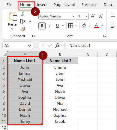
For this method, we’ll use a simple dataset of names with two columns (Column A and Column B). The common values will be shown in column C by comparing the two columns.
To compare two columns and return common values, we’ll combine the IF and COUNTIF functions. In this case, the COUNTIF function determines how many times a value from column A appears in column B. The IF function determines what should be displayed by using that number. If it is greater than 0, it returns the common value; otherwise, it returns a blank.
Steps:
➤ Click on cell C2 and write this formula:
=IF(COUNTIF(B:B, A2), A2, "")
➤ Press Enter and see the first common name in the cell C2.
➤ Drag down to see the other common names. Name list 1 is compared with name list 2.
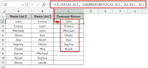
Using FILTER Function
In this method, we will use the same namelist dataset. We’ll combine the FILTER function with the MATCH and ISNUMBER functions.
The MATCH function finds each name from Column A that is present or not in Column B. If the name is found, it produces a number; otherwise, it will show an error. The matched result is changed to TRUE, and the unmatched results to FALSE by the ISNUMBER function. Using that TRUE/FALSE logic, the matched names are extracted from Columns A and Column B by the FILTER function. A blank-free list of common values will be shown in Column C as an output.
Steps:
➤ Click on cell C2 and write this formula:
=FILTER(A2:A11, ISNUMBER(MATCH(A2:A11, B2:B11, 0)))
➤ Press Enter and see all the common names in Column C. It shows all the common names in a dynamic array.
Using Conditional Formatting
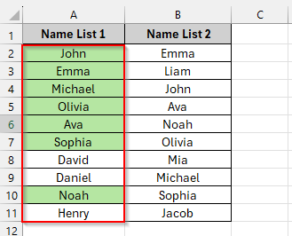
Using the same dataset of names from Columns A and B, we will use a COUNTIF function inside the Conditional Formatting rule. The COUNTIF function checks how many times a value from Column A appears in Column B. Excel will automatically highlight that cell if the count is more than zero. That means the value is present in both columns. After comparing two columns, common names will be highlighted in color.
Steps:
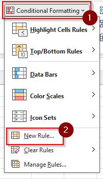
➤ Select Column A > Home
➤ Click on Conditional Formatting > New Rule.
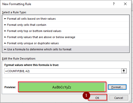
➤ Choose “Use a formula to determine which cells to format” then
set the formula in the formula box =COUNTIF(B:B, A1) and click the Format button.
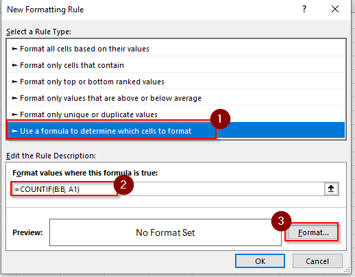
➤ Click on the Fill tab, set a colour, and click OK.
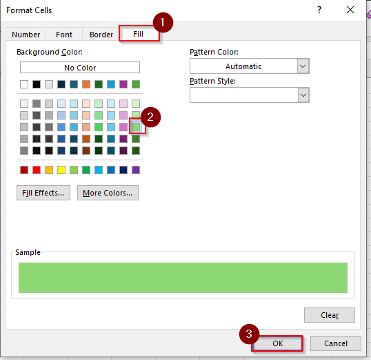
➤ You can see the preview of the color, and click OK
➤ Common names are highlighted in column A. You can do it for column B as well.
VLOOKUP Function to Return Common Matches
In this method, we’ll check each name in Column A that exists in Column B by using the VLOOKUP function.
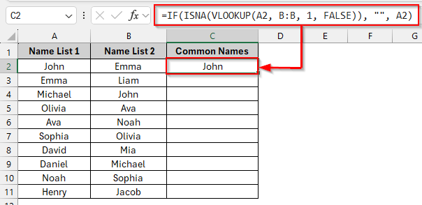
The VLOOKUP function searches for the value from Column A in Column B, and if a matching value is found, it returns that value; otherwise, the ISNA function finds the error, and the IF function replaces it with a blank. As an output, you can see the common names in Column C.
Steps:
➤ Click on cell C2 and write this formula:
=IF(ISNA(VLOOKUP(A2, B:B, 1, FALSE)), "", A2)
➤ Press Enter and see the first common name in C2
➤ Drag down to see the other common names. Here, the VLOOKUP function also compares the name list 1 with the name list 2.
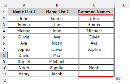
Using the XLOOKUP Function
We’ll use the XLOOKUP function along with the IFERROR function here to compare two columns and return common values. XLOOKUP searches each value from Column A inside Column B. If it finds a common value, it returns the value; if it doesn’t, it gives an error. To avoid showing errors in the result, the IFERROR function replaces the error with a blank. As an output, we will get the common values, while the unmatched values are left empty.
Steps:
➤ Click on cell C2 and write this formula:
=IFERROR(XLOOKUP(A2, B:B, B:B), "")
➤ Press Enter and see the first common name in the cell C2
➤ Then drag down the cell, and you can see the common names in Column C

Frequently Asked Questions
Is it possible to return common values from both directions?
Yes, you can return common values from both directions. You have to apply the same formula logic in both directions. One formula checks if column A values are in column B, and another formula checks if column B values are in column A.
What are the reasons for getting the #N/A error?
If you get a #N/A error, that means that the value from one column does not exist in the other column.
How can I get common values in both columns with no blanks?
Using the FILTER function =FILTER(A2:A11, ISNUMBER(MATCH(A2:A11, B2:B11, 0))). You can get a list of common values with no blanks.
If there are duplicate values, will the formula still function?
“Yes.” Formulas will return each match exactly as it is. Use Excel 365‘s UNIQUE function or manually remove duplicate results.
Wrapping Up
In this article, we have discussed five different ways to compare two columns and return common values in Excel. By comparing two columns, you can know the matched values in both columns. Feel free to download the practice file and share your thoughts and suggestions.