Sometimes, you need to break a long string of text or numbers into smaller parts in Excel. For example, if your product code is like ABC123XYZ789, and you want to split it into 3 characters (ABC, 123, XYZ, 789). There is no built-in tool to split a string by length, but we can do this by using formulas and Power Query tools.
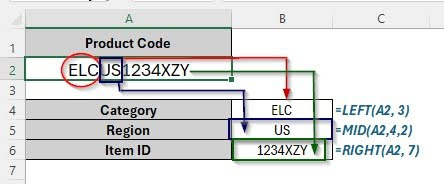
To split the “ELCUS1234XZY” string by length using the LEFT, MID, and RIGHT functions, follow these steps.
➤ Select cell B4 and write this formula: =LEFT(A2, 3)
➤ Press Enter, and you will see the category is “ELC”
➤ Select cell B5 and write this formula: =MID(A2, 4, 2)
➤ Press Enter, and you will see the Region is “US”
➤ Select cell B6 and write this formula: =RIGHT(A2, 7)
➤ Press Enter, and you will see the Item ID is “1234XZY”
In this article, we’re going to know different suitable methods to split a string by length in Excel, which include using LEFT, MID and RIGHT functions, using Power Query, using Flash Fill, and Text to Column Options.
Using LEFT, MID, and RIGHT Functions
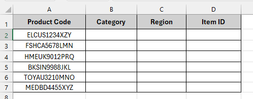
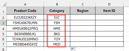
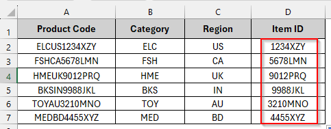
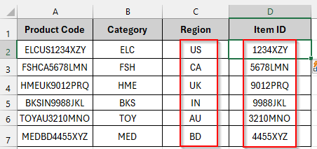
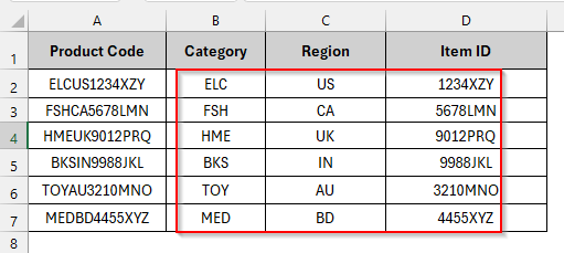
In the following dataset, we have 12 character product codes which will be split into Category, Region and Item ID. To split the product code into 3-character categories, we will use the LEFT function. By using the MID function, the Region will be 2 characters in length, and the Item ID will be 7 characters in length by using the RIGHT function.
Follow these steps to split the product code into a 3-character-long Category name by using the LEFT function.
Steps:
➤ Select cell B2 and write this formula:
=LEFT(A2, 3)
➤ Press Enter, and you will see that the product code is split into a 3-character-long Category name.
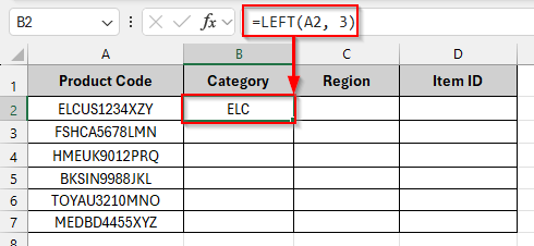
➤ Drag down the formula to see the other split product codes to the category name.
Follow these steps to split the product code into a 2-character-long Region name by using the MID function.
Steps:
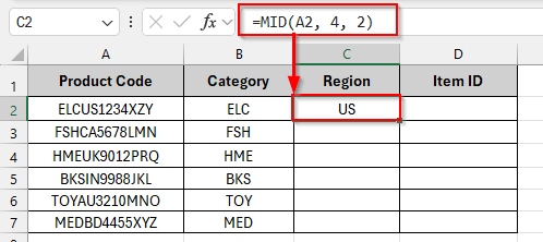
➤ Select cell C2 and write this formula:
=MID(A2, 4, 2)
➤ Press Enter, and you will see that the product code is split into 2-character-long Region names.
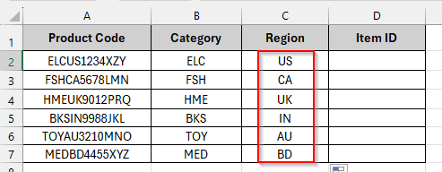
➤ Drag down the formula to see the other split product codes to the Region name.
Follow these steps to split the product code into a 7-character-long Item ID by using the RIGHT function.
Steps:
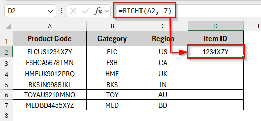
➤ Select cell D2 and write this formula:
=RIGHT(A2, 7)
➤ Press Enter, and you will see that the product code is split into a 7-character-long Item ID.
➤ Drag down the formula to see the other split product codes to the Item ID.
Using Power Query to Split String by Length
Power Query is a powerful tool in Excel that helps to split strings easily based on their position. By using the “Split Column by Number of Characters” feature in Power Query, you can split a string into multiple parts in just a few steps. After that, you can load the split results directly into your worksheet.
Steps:
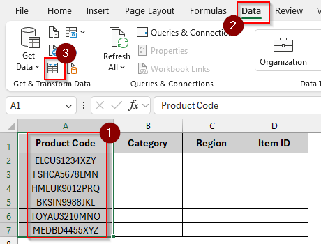
➤ Select Column A > click Data > From Table/Range
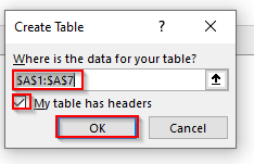
➤ The Create Table pop-up message will show. Check the “My table has headers” option and click OK.
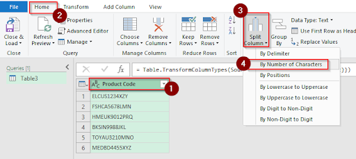
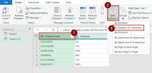
➤ In Power Query, select Product Code, click Home > Split Column > By Number of Characters
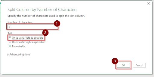
➤ Enter “3” in the Number of characters box. Choose the “Once, as far left as possible” option and click OK.
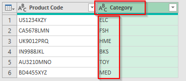
➤ You will see that the product code is split into 3 characters. Rename this column as “Category”.
➤ Repeatedly, select Product Code > Split Column > By Number of Characters to split the product code into a 2-character-long Region name.
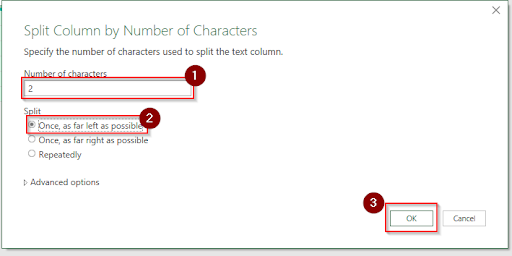
➤ Enter “2” in the Number of characters box. Choose the “Once, as far left as possible” option and click OK.
➤ You will see that the product code is split into 2 characters long and the remaining part is 7 characters long. Rename these columns as “Region” and “Item ID” and then click Close & Load.
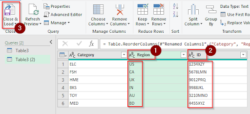
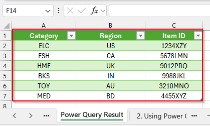
➤ Now, you can see that the split table will be loaded into another sheet as a result.
Using Flash Fill to Split Text by Pattern
Flash Fill can automatically detect patterns in your data and fill in the rest for you. You just need to type how you want the first result to look, and then, after clicking the Flash Fill, it can fill the rest of the cells.
Steps:
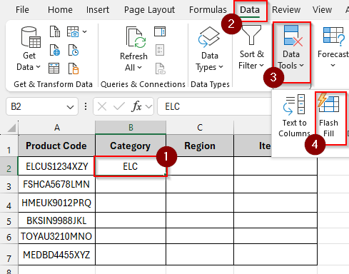
➤ Select cell B2 and type “ELC”
➤ Click on cell B3 and click Data> Data Tools > Flash Fill
➤ Excel will automatically fill the Category Column like cell B2.
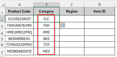
➤ Repeat the same for the Region and Item ID column.
Using the Text to Columns Option
Excel’s Text to Columns is a built-in tool to split data from one column into multiple columns. By using this fixed-width option, you can manually define the split positions, where the split result will be shown and create break lines at the desired position to split a string by length.
Steps:
➤ Select the Product Code column
➤ Click Data > Data Tools > Text to Columns
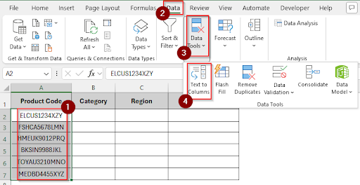
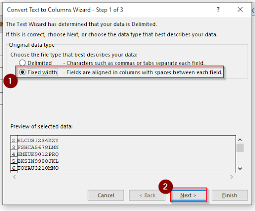
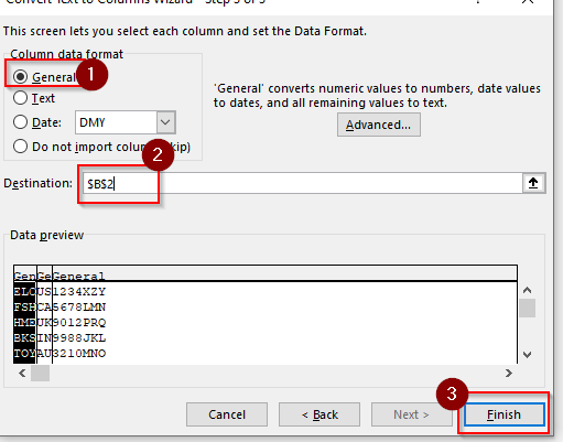
➤ Choose Fixed Width > click Next
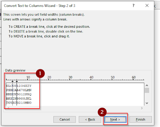
➤ Click to insert break lines after character 3 and character 2, and then click Next
➤ Select the column data format option to General, enter the destination as $B$2, and then click Finish.
➤ Now you can see that the product code is split into Category, Region and the Item ID.
Frequently Asked Questions
Is it possible to reverse a split created with Text to Columns?
No, the original column gets overwritten once the data has been divided using Text to Columns. Keep a backup copy of your data before using it.
Which method is the best for big datasets?
Power Query is the most effective way to handle large and updated data. Also, you can update the split results anytime when your data changes.
Will my original data be replaced by Power Query?
No, your original data will be preserved by Power Query while loading the updated data into a new sheet.
Wrapping Up
In this article, we have discussed four distinct methods step by step for splitting a string by length in Excel. Feel free to download the practice file and share your thoughts and suggestions.