
In large sheets, when we scroll down, we feel the necessity to freeze certain rows and columns to keep the headers and section labels visible. It helps to understand data and enter it into cells without making mistakes. Freezing multiple rows improves navigation of the sheet and maintains the context of the data. This feature saves time and makes a spreadsheet more user-friendly. In this article, we will show you how to freeze multiple rows in Google Sheets.
Google Sheets only allows freezing contiguous rows. It means you can freeze multiple rows, up to a specified row, starting from the first row. You can not freeze separate or specific rows in the middle of the sheet.
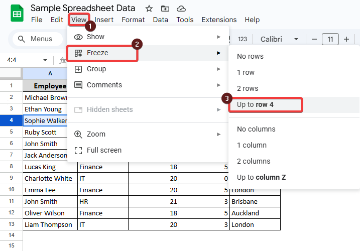
Suppose you want to freeze the first four rows of a spreadsheet. You can easily do that using the menu bar of Google Sheets. Read the steps below to learn how to do that.
➤ Select the row up to which you want to freeze.
➤ Go to View >> Freeze >> Up to row 4.
In this way, multiple rows will be frozen.

What Does It Mean to Freeze Rows in Google Sheets?
Freezing rows means locking the position of multiple rows in their initial position. We do this to keep the rows always visible while scrolling down Google Sheets. Sometimes we need to freeze the rows to see the headers and subheaders of the sheet. It helps us to navigate easily in complex datasets.
In this article, we will learn how to freeze multiple rows in Google Sheets. We will show two simple methods of doing it. You can use the menu bar option, or you can freeze rows simply by dragging a line in Google Sheets.
Using the Menu Bar Option to Freeze Rows in Google Sheets
It’s the most common and well-known method to freeze multiple rows in Google Sheets. Whether you want to freeze a single row or a couple of rows, you can easily do that from the menu bar option. Follow the steps below to learn how to do that.
Steps:
➤ Click on the row number up to which you want to freeze.
➤ Select View >> Freeze >> Up to row 4.
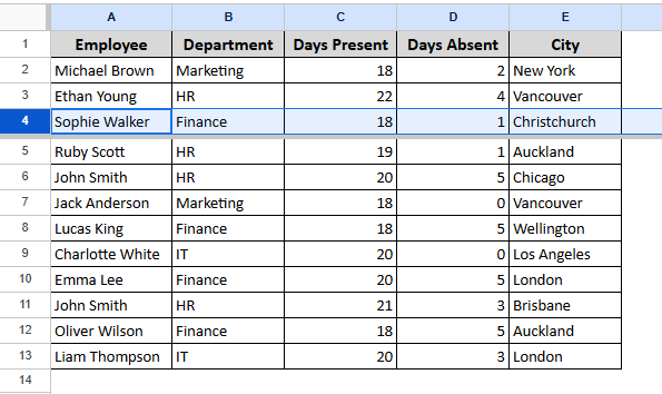
You will see a thick gray line under the selected row. This means your rows are frozen.

Using the Drag-Freeze Line to Freeze Multiple Rows
This method is the quickest way to freeze rows. But it is not as common and well-known as the previous one. Follow the steps to learn how to do that. It’s especially handy if you prefer using your mouse instead of navigating through the menu options. Using this method, you can quickly drag and lock rows in just a second. Follow the steps below to learn the method.
Steps:
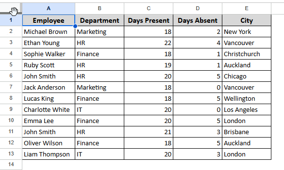
➤ Take the cursor to the gray line in the top left corner of the sheet, above the first row number.
You will see a hand icon similar to the one shown in the following image.
➤ Drag down the icon to your desired position. You will see the grey line going down with it.
All the rows above the grey line will be frozen.
How to Unfreeze Rows in Google Sheets?
It is also important to know how to unfreeze rows after freezing multiple rows. Because sometimes you may only need the frozen rows temporarily. After analyzing or editing, you can easily unfreeze the headers. Unfreezing restores your sheet to the normal scrolling mode. It provides the user with a full view of all rows, without any locked headers at the top. The process to unfreeze rows is very simple. Read the following steps to know that.
Steps:
➤ Select View >> Freeze >> No rows.
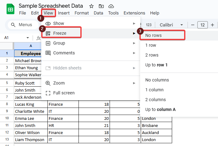
It will unfreeze the rows, as shown in the following image.
You can also drag the gray freeze line back to its original position at the top-left corner of the sheet to unfreeze rows manually.
Frequently Asked Questions (FAQs)
Can I freeze separate, non-adjacent rows in Google Sheets?
No, Google Sheets does not allow freezing non-contiguous rows. You can only freeze adjacent, contiguous rows. For example, you can freeze the first three rows together, but you cannot freeze row 1 and row 10 separately.
How can I unfreeze rows in Google Sheets?
To unfreeze rows, go to the top menu and click View >> Freeze >> No rows. This will instantly remove the frozen section, allowing you to scroll through the sheet normally.
Can I freeze both rows and columns at the same time?
Yes, you can freeze both rows and columns simultaneously in Google Sheets. To do this, click on the cell that is just below the last row and just to the right of the last column you want to freeze. Then go to View >> Freeze and select the appropriate rows and columns.
Is there a limit to the number of rows I can freeze?
No, there is no limit to the number of rows you can freeze. You can freeze as many rows as you like, but they must be contiguous starting from row 1.
Wrapping Up
Freezing multiple rows in Google Sheets is a very easy task. We often need to freeze rows in Google Sheets to easily maintain our data and keep the headers visible. After reading this article, we hope you can do it effortlessly now. It will help you to input or check your data efficiently.

