Both INDEX-MATCH and XLOOKUP are two powerful lookup functions in Excel used to find data from a specific range. You can use them for exact matches, approximate matches, two-way lookups, binary searches, left lookups, etc. However, the functions differ in syntax, complexity, error handling methods, compatibility, and other capabilities.
For example, you can replace an error with a blank or text with XLOOKUP. To do the same with INDEX+MATCH, you must include the IFERROR function, which complicates the syntax.
➤ XLOOKUP relies on a single syntax to perform a wide range of actions including vertical and horizontal search, wildcard lookups, binary search, two-way lookups, etc. INDEX MATCH combines two functions to achieve the same results.
➤ While INDEX MATCH requires data alterations or added functions for approximate matches and error handling, XLOOKUP has these built-in in the syntax. Moreover, INDEX MATCH can’t find the last match via reverse search like XLOOKUP.
➤ INDEX MATCH is universal for all Excel versions and offers great flexibility for advanced searches. Unfortunately, XLOOKUP is only available in Excel 365/2021.
In this article, we’ll compare XLOOKUP vs INDEX MATCH, including all the similarities and differences between the two lookup methods.
Definitions of XLOOKUP vs INDEX-MATCH Formula in Excel
Let’s start by understanding what the functions do and how they work.
What Is XLOOKUP?
XLOOKUP is a comparatively new, single function that searches a range or array, finds the correct match, and returns the corresponding result. In Excel, it replaces VLOOKUP, HLOOKUP, and INDEX MATCH.
What is INDEX MATCH?
The INDEX function returns a value from a range based on row and column numbers. On the other hand, MATCH returns the position of a lookup value in a range. When combined, MATCH finds the row/column number and INDEX extracts the cell value using that number, offering a flexible lookup option.
Syntax Comparison Between XLOOKUP and INDEX-MATCH
What sets the two lookup methods apart is the syntax of the used functions. Below are the details:
Syntax of the XLOOKUP Function
A basic XLOOKUP formula looks like this:
=XLOOKUP(lookup_value, lookup_range, return_range, [if_not_found], [match_mode], [search_mode])
Here, the first 3 arguments are mandatory and they represent:
- lookup_value: The value you want to search for.
- lookup_range: The range/array where Excel looks for the value.
- return_range: The range/array from which to return the result.
For flexibility, the last arguments are added, representing the following:
- [if_not_found]: The message/value to return if no match is found.
- [match_mode]: Set up how to match the value. You can enter 0 for an exact match (default). Use -1 for an exact match or the next smaller match. Enter 1 for an exact match or the next larger. Finally, you can use 2 for wildcard matches (\➤, ?).
- [search_mode]: For search direction, use 1 to search first to last (default) or -1 for last to first.
Syntax of the INDEX-MATCH Formula
When combined, a formula with INDEX MATCH will have the following arguments:
=INDEX(return_range, MATCH(lookup_value, lookup_range, match_type), no_of_column)
Let’s find out what the different parts of the syntax do:
INDEX Function
- return_range: The range/array of cells from which we want to extract a value. It can be multiple rows and multiple columns.
- MATCH(lookup_value, lookup_range, match_type): Returns the row number inside the range where the lookup value is found.
- no_of_column (optional): A number that specifies which column of the range/array to return the value from.
MATCH Function
- lookup_value: The value you are searching for.
- lookup_range: The column (or row) in which Excel looks for the lookup value.
- match_type (optional): Defines how Excel matches the value. Inserting 0 finds an exact match. Use 1 to find the largest value less than or equal to the lookup_value (array must be sorted ascending). Finally, -1 finds the smallest value greater than or equal to the lookup_value (array must be sorted descending).
Compatibility, Readability, and Speed of XLOOKUP vs INDEX-MATCH
Some basic differences between the two lookup methods are as follows:
Compatibility
Although XLOOKUP is a great new addition to the lookup functions, it’s only available in Excel 365, Excel 2021, and newer versions. For all older Excel versions, you must use INDEX MATCH for flexible lookups.
Formula Readability
As INDEX MATCH combines two functions, it can be slightly complex for beginners. On the other hand, XLOOKUP is a single and more intuitive function with fewer arguments and built-in flexibility.
Speed
When used as array formulas for thousands of rows, XLOOKUP works a little faster than INDEX MATCH. However, the difference is ignorable and both functions take a few seconds to find a value from large datasets.
Basic Lookups Using XLOOKUP vs INDEX MATCH
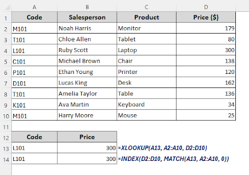
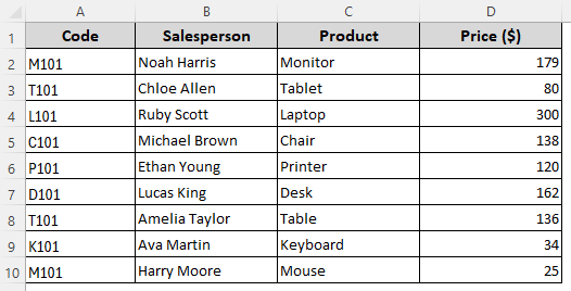
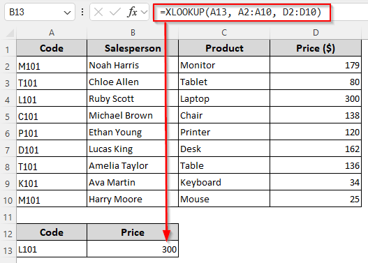
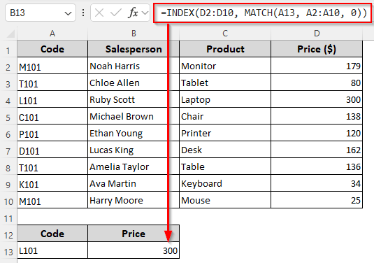
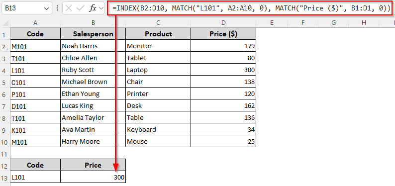
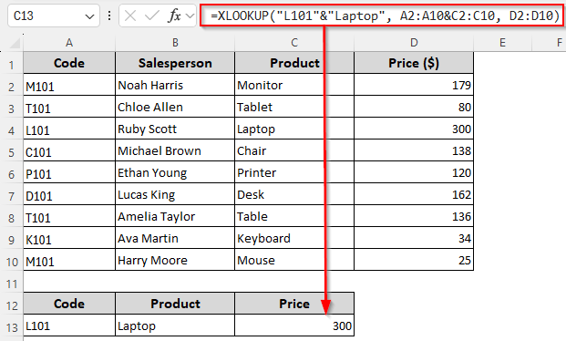
For visual aid, we’ll use a sample dataset with product codes, sales agent names, product names, and prices. Our lookup value is the product code L101 from Column A (A1:A10). We want to get its price ($300) from the corresponding cell in the return Column D (D1:D10).
Let’s look at some basic lookup methods using XLOOKUP and INDEX MATCH:
Lookup with Cell Reference
First, we put the lookup value in cell A13. Now, use any of the insert any of the following formulas in a cell where we want to return the price:
XLOOKUP Function
=XLOOKUP(A13, A2:A10, D2:D10)
➤ Change the lookup range A2:A10, return range D2:D10, cell reference A13 according to your dataset.
➤ Press Enter.
INDEX MATCH Functions
=INDEX(D2:D10, MATCH(A13, A2:A10, 0))
➤ Replace the ranges and cell reference as required.
➤ Click Enter.
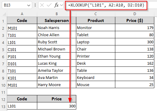
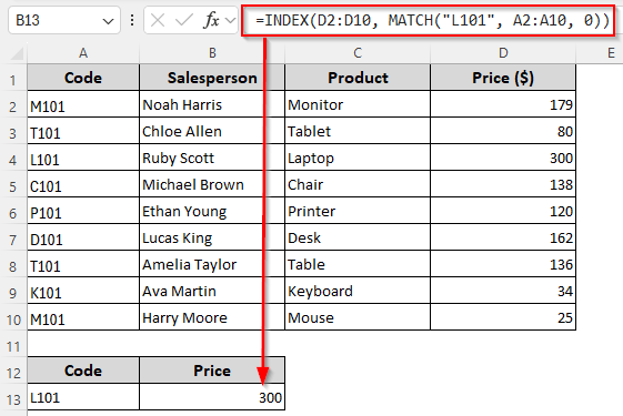
Lookup with Direct Value (Text)
To directly use the lookup value instead of using a cell reference, use the following formulas:
XLOOKUP Function
=XLOOKUP("L101", A2:A10, D2:D10)
➤ Here, A2:A10 is the lookup range, D2:D10 is the return range, and L101 is the lookup value. Replace them as needed.
➤ Press Enter.
INDEX MATCH Functions
=INDEX(D2:D10, MATCH("L101", A2:A10, 0))
➤ Change the ranges and lookup value as per your data.
➤ Click Enter.
Finding Approximate Matches with XLOOKUP vs INDEX MATCH
With XLOOKUP, no alterations are required in your dataset to find the next smaller or larger value when the exact match isn’t found.
However, if you want to find the next smaller value with INDEX MATCH, you must sort your data in ascending order (smallest to largest). To find the next larger value, your data must be sorted in descending order (largest to smallest).
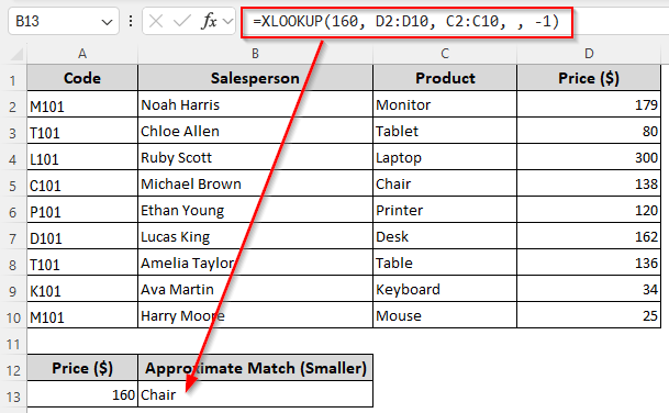
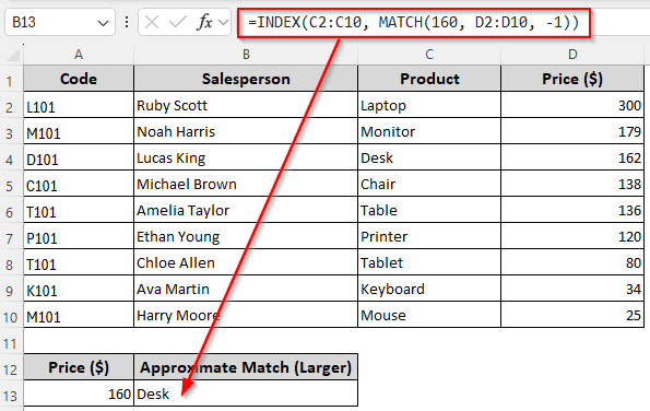
In this example, we’ll find the product name from Column C (C1:C10) for the price $160 in Column D (D1:D10). Let’s get into the details:
Find the Next Smaller Value
➤ In a cell where you want to return the found value, insert any of these formulas:
XLOOKUP Function
=XLOOKUP(160, D2:D10, C2:C10, , -1)
➤ Replace the lookup range D2:D10, return range C2:C10, and lookup value 160 according to your dataset.
➤ Click Enter.
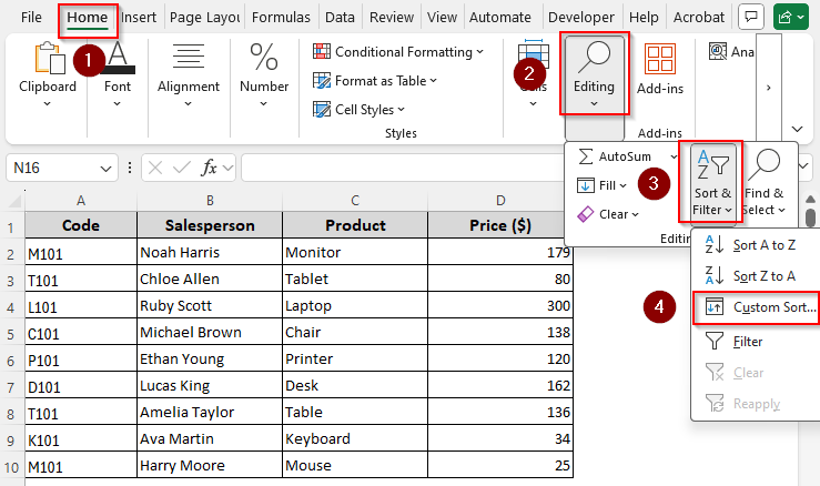
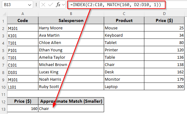
INDEX-MATCH Formula
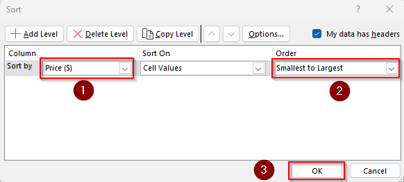
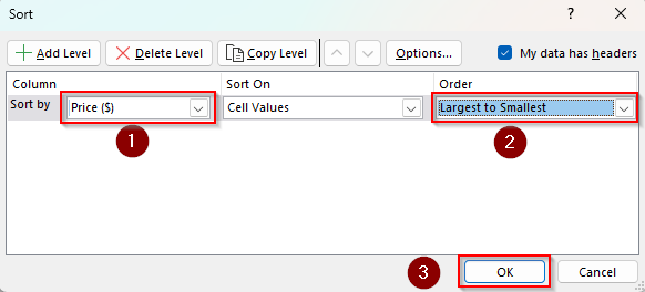
➤ First, sort your data in an ascending order by going to the Home tab >> Sort & Filter group >> Custom Sort.
➤ From the Sort window, select the Price ($) column from the Sort By drop-down and Smallest to Largest from the Order drop-down. Press Ok.
➤ Now, insert the following formula where you want the returned value:
=INDEX(C2:C10, MATCH(160, D2:D10, 1))
➤ Change the ranges and lookup value as needed.
➤ Press Enter.
Find the Next Larger Value
Enter any of the following formulas in a cell selected for the returned value:
XLOOKUP Function
=XLOOKUP(160, D2:D10, C2:C10, , 1)
➤ Replace the ranges and lookup value as required and click Enter.

INDEX-MATCH Formula
➤ To sort your data in a descending order, go to the Home tab >> Sort & Filter group >> Custom Sort. In the Sort dialog box, choose the Price ($) column from the Sort By options and Largest to Smallest from the Order options. Click Ok.
=INDEX(C2:C10, MATCH(160, D2:D10, -1))
➤ Change the ranges and lookup value if required and click Enter.
Reverse Search/Last Match Lookup Using the XLOOKUP vs INDEX MATCH Functions
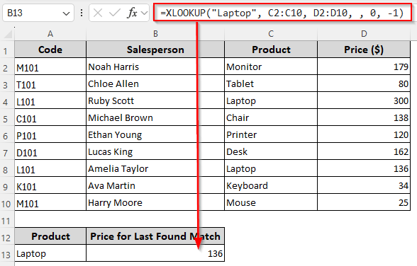
While INDEX MATCH can only search from top to bottom, XLOOKUP works in all directions including bottom to top. It’s particularly helpful when you’re looking for the last matching value from a range. Here’s how to reverse search with XLOOKUP:
➤ To find the price of the last found match for Laptop, enter the following formula:
=XLOOKUP("Laptop", C2:C10, D2:D10, , 0, -1)
➤ Here, Laptop is the lookup value, C2:C10 is our lookup range, and D2:D10 is the return range. Change them as required.
➤ Click Enter.
Two-Way Lookup with XLOOKUP vs INDEX MATCH Functions
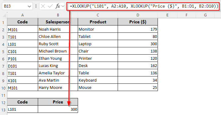
A two-way lookup is used to find a value at the intersection of a specific row and a specific column. Both XLOOKUP and INDEX MATCH can do it, but INDEX MATCH is usually cleaner. With XLOOKUP, we need to nest two XLOOKUP functions as explained below:
➤ Here, we’ll look for the product price from the Price ($) column for the product code L101. We’ll use the following formulas:
XLOOKUP Function
=XLOOKUP("L101", A2:A10, XLOOKUP("Price ($)", B1:D1, B2:D10))
➤ Our lookup value is L101 and lookup range is A2:A10. B1:D1 is our return range with the column headings and B2:D10 excludes the headers. The column containing the return value is titled Price ($). Change these values as needed.
➤ Click Enter.
INDEX-MATCH Functions
=INDEX(B2:D10, MATCH("L101", A2:A10, 0), MATCH("Price ($)", B1:D1, 0))
➤ Replace the ranges, column heading, and lookup value as required.
➤ Press Enter.
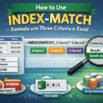
Lookup Based on Multiple Conditions with XLOOKUP vs INDEX MATCH
Although you can search for a value based on multiple conditions using XLOOKUP and INDEX MATCH, using the XLOOKUP function is easier as the syntax is simpler. Here’s how to use these functions with multiple conditions:
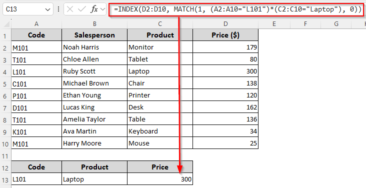
➤ To find the selling price for a Laptop matching the code L101, use any of the following formulas:
XLOOKUP Function
=XLOOKUP("L101"&"Laptop", A2:A10&C2:C10, D2:D10)
➤ Replace the lookup values L101&Laptop, lookup ranges A2:A10&C2:C10, and return range D2:D10 according to your dataset.
➤ Click Enter.
INDEX-MATCH Functions
=INDEX(D2:D10, MATCH(1, (A2:A10="L101")*(C2:C10="Laptop"), 0))
➤ Replace the ranges and values as required.
➤ For Excel 365 or 2021, press Enter . If you’re using an older version, click Ctrl + Shift + Enter .
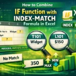
Comparing XLOOKUP vs INDEX MATCH Functions for Error Handling
As XLOOKUP has an optional [if_not_found] argument, you can directly handle errors with it without any extra functions. However, with INDEX MATCH, you must wrap your formula with IFERROR to handle errors. Let’s get into the details:
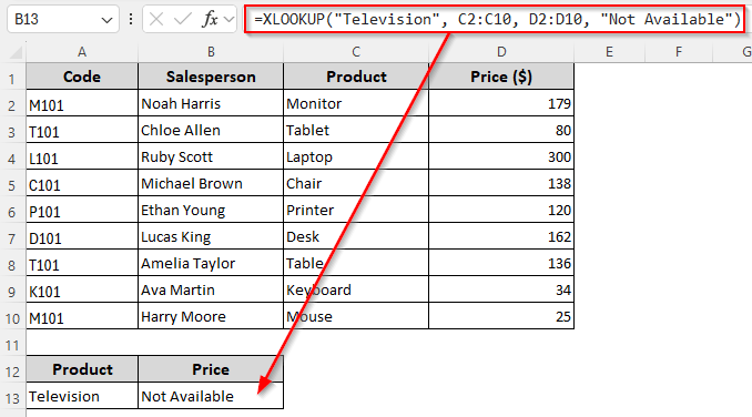
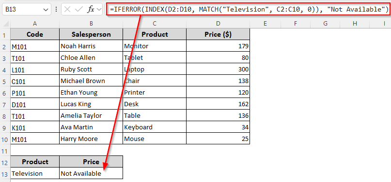
➤ We’ll look for the Television in Column C and return its price from Column D. As we don’t have the value in our data range, Excel will return an #N/A error. Our goal is to replace it with Not Available. For this, we’ll use the formulas given below:
XLOOKUP Function
=XLOOKUP("Television", C2:C10, D2:D10, "Not Available")
➤ Change the lookup range C2:C10, return range D2:D10, and error replacement text Not Available according to your needs. To return a blank instead of text, use “”.
➤ Press Enter.
INDEX-MATCH Functions
=IFERROR(INDEX(D2:D10, MATCH("Television", C2:C10, 0)), "Not Available")
➤ Replace the ranges and texts as needed.
➤ Press Enter.
XLOOKUP vs INDEX-MATCH at a Glance
Some key comparable aspects between the lookup methods are as follows:
| Comparable Aspects | XLOOKUP | INDEX-MATCH |
|---|---|---|
| Available in | Excel 365 and 2021 only | All Excel versions |
| Error Handling | In-built options in syntax | Requires IFERROR |
| Reverse Search (Bottom to Top) | Yes | No |
| Two-Way Lookup | Yes | Yes |
| Speed | Slightly faster | Slower than XLOOKUP |
| Lookup with Multiple Conditions | Included in Syntax, no sorting required | Works only with sorted data |
| Approximate Match | Included in Syntax, no sorting required | Works only with sorted data |
| Spill Arrays | Yes | No |
| Wildcard Search | Yes | Yes |
Frequently Asked Questions
What are the limitations of XLOOKUP?
While XLOOKUP is very powerful, it can become slow for extremely large workbooks as it always searches the entire array. Unlike Power Query or INDEX/MATCH combos, XLOOKUP can’t directly return multiple non-adjacent columns at once. When using the fast binary search mode (search_mode = 2 or -2), the data must be sorted, otherwise results are unreliable.
Can you use wildcards with INDEX MATCH and XLOOKUP?
Yes, both support wildcards only when the match type is set to exact match. If you want to look for a value starting with App (like Apple, Application, etc.), use any of the following formulas:
=XLOOKUP(“App*”, C2:C10, D2:D10, “Not Found”, 0)
Or,
=INDEX(D2:D10, MATCH(“App*”, C2:C10, 0))
Adjust the lookup range C2:C10, return range D2:D10, and lookup value App* as needed.
Which is better VLOOKUP or INDEX MATCH?
INDEX MATCH is better than VLOOKUP as it can look left or right, while VLOOKUP can only look right. Inserting/deleting columns doesn’t break INDEX MATCH, but it breaks VLOOKUP since it relies on a fixed column index. Also, INDEX MATCH allows multi-criteria lookups and you can combine them with other functions.
Concluding Words
XLOOKUP combines the flexibility of INDEX+MATCH with simpler syntax and additional features. Yet, INDEX+MATCH remains valuable for compatibility with older files and in performance-critical situations with very large datasets. While choosing between them, consider your search intention, Excel version, and the outcome you want.