
A contingency table or crosstabs shows the frequency distribution of two categorical variables. You can use Excel features and functions to easily make a contingency table.
➤ A contingency table shows the number of observations that fall into each category.
➤ Using PivotTable: Insert >> PivotTable >> Choose Fields >> Field Settings >> Count.
➤ Using formula: =COUNTIFS(criteria_range1, criteria1, criteria_range2, criteria2)
➤ To update changes to the PivotTable: Right-click >> Refresh.
In this article, we’ll learn about the contingency table or crosstabs and how we can make them using the PivotTable and COUNTIFS function in Excel.
What is a Contingency Table?
A contingency table (cross-tabulation or crosstabs) displays the frequency distribution of two categorical variables by showing the number of observations that fall into each category. Contingency tables are useful for analyzing the relationship between two categorical variables
Using PivotTable to Create a Contingency Table in Excel
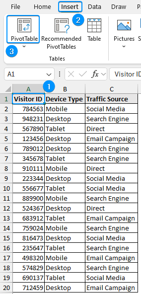
This dataset contains information about website visitors based on the device type and traffic source. Let’s use the PivotTable to make a contingency table or crosstab.
Steps:
➤ Select any cell within the dataset >> Insert >> PivotTable.
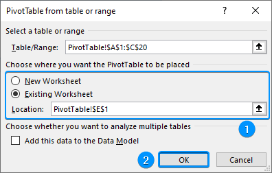
➤ Choose Existing Worksheet >> Location (E1) >> OK.
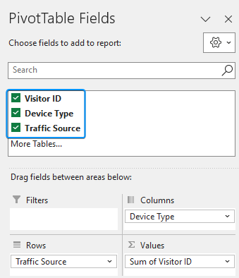
➤ Drag the visitor ID field into the Values area, the device type field into the Columns area, and the traffic source into the Rows area.
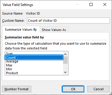
➤ Click the drop-down arrow beside Sum of Visitor ID >> Value Field Settings.
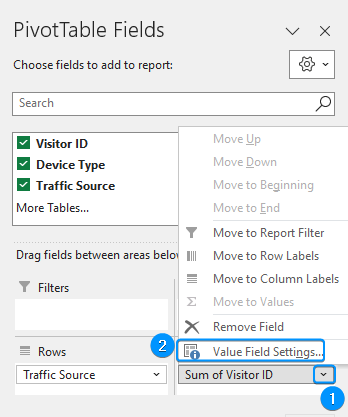
➤ Choose the Count option >> OK.
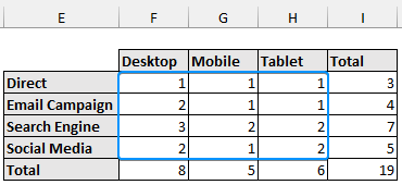
➤ The contingency table will be generated automatically.
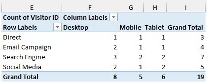
➤ Row Total:
3 visitors visited the website directly.
4 visitors visited the website through email campaign.
7 people visited the website from a search engine.
5 people visited the website through social media.
➤ Column Total:
8 visitors used a desktop.
5 visitors used a mobile.
6 visitors used a tablet.
➤ Desktop Column:
1 visitor used a desktop to visit the website directly.
2 visitors used a desktop to visit the website through email campaign.
3 visitors used a desktop to visit the website using a search engine.
2 visitors used a desktop to visit the website through social media
➤ The Mobile and Tablet columns will have similar interpretations.
Contingency Table with COUNTIFS Function
You can use Excel’s COUNTIFS function to quickly make a crosstab.
Steps:
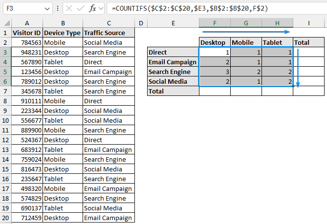
➤ Select the output cell (F3) and enter the formula.
=COUNTIFS($C$2:$C$20,$E3,$B$2:$B$20,F$2)
➤ Pressing the F4 key once locks both the row and column references.
➤ Pressing F4 a second time locks only the row reference.
➤ Pressing it a third time will lock only the column reference.
➤ Pressing for the fourth time removes the dollar sign altogether.
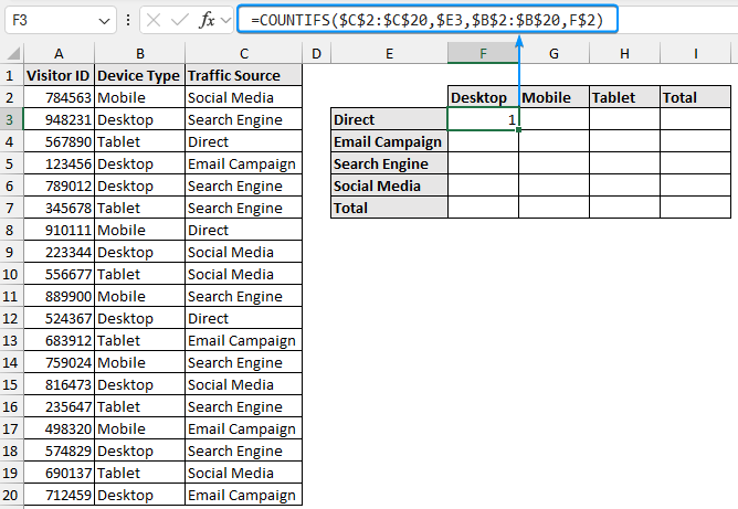
➤ Drag the Fill Handle tool across and then downward to copy the formula.
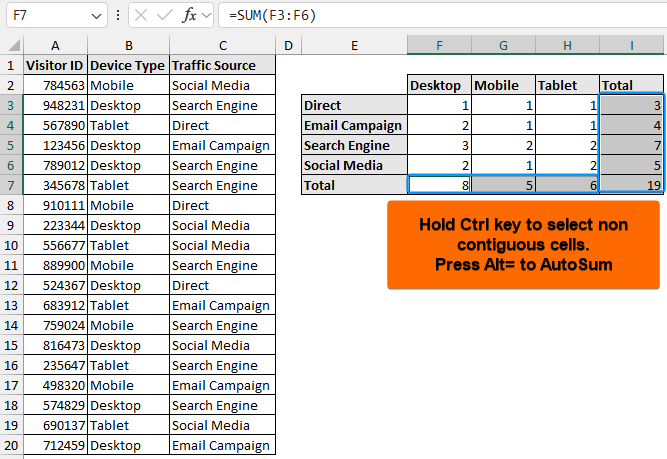
➤ Hold the Ctrl key >> Select the row totals (I3:I7) and column totals (F7:H7) >> Press Alt= to get the totals.
FAQ
How do I make a contingency table in Excel?
➤ Using PivotTable: Select data >> Insert >> PivotTable >> Choose Fields >> Set Value Field Settings to Count.
➤ Using formula: =COUNTIFS(criteria_range1, criteria1, criteria_range2, criteria2)
What are contingency tables known as in Excel?
Contingency tables are also known as crosstabs.
What are the three types of contingency tables?
The three types of contingency tables are: joint, marginal, and conditional.
How to customize the layout and format of my contingency table?
Select any cell inside the PivotTable and the contextual Design tab will appear. You can change the style, layout, add-remove subtotals, grand totals, etc. to customize the contingency table.
How to update the contingency table if my data changes?
You can update the contingency table by refreshing the PivotTable. Right-click on the PivotTable and select Refresh or click the Refresh button in the PivotTable Analyze tab.
Wrapping Up
In this tutorial, we’ve learned about contingency tables or cross tabs and how to make a contingency table in Excel. Feel free to download the practice file and let us know which method you like the most.