Calculated fields are often used in Excel to calculate new values from the existing fields. However, calculated fields are usually done for rows in a pivot table. Although it’s rare, sometimes you just need to create new columns based on existing column values, typically to filter the data. The column headers in a pivot table cannot be calculated using a calculated field, but we can use calculated items to do so. In this article, we will learn how to mimic a calculated field based on column values.
➤ Select a cell of the column that you want to calculate.
➤ Go to PivotTable Analyze tab on the ribbon, and head to Calculations > Fields, Items, & Sets > Calculated Item.
➤ Write the new column name (4th Week in this case) in the edit box called Name.
➤ Write the following formula in the Formula edit box, change according to your needs:
=’4/20/2025’+’4/22/2025’+’4/24/2025’+’4/26/2025′
➤ Click Add and OK to add the new column to the pivot table.
Column Values cannot usually be used for calculated fields, but we can use a workaround to calculate column values. In this article, we will walk you through the process of applying the workaround step by step.
Steps for Creating a Calculated Field Based on Column Values
To demonstrate the process, we created a pivot table from sales data. There are product names, names of the salespersons, the units they sold, and the due dates of their sales quota. We have populated the dates in the columns, and we would like to create a calculated column for the fourth week of April 2025 that displays the sales data for that week. Follow the steps below to do so:
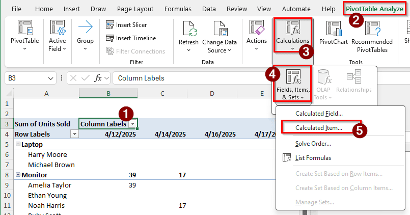
Step 1: Prepare the Calculation
Calculated fields cannot work with column values. Instead, as a workaround, we will use calculated items. First, we need to select which fields will be used for calculation, and go to the appropriate menu to add the calculated item.
➤ Select a date cell of the pivot table.
➤ Go to the PivotTable Analyze tab on the ribbon.
➤ From the Calculations group, go to Fields, Items, & Sets > Calculated Item.
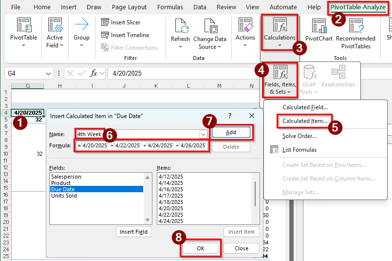
Step 2: Insert the Required Formula
After the first step, we will see a new window that will help us add the calculated item. We need to insert some values to make it work. Follow the instructions below:
➤ In the window, change the “Name:” field to 4th Week.
➤ In the Formula field, write the following formula:
='4/20/2025' +'4/22/2025' +'4/24/2025' +'4/26/2025'
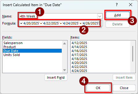
➤ Press Add and OK afterwards.
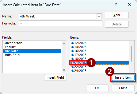
➤ If you don’t feel like writing the big formula, you can also select certain dates from the right panel one by one and click Insert item, then add the pluses (+) manually.
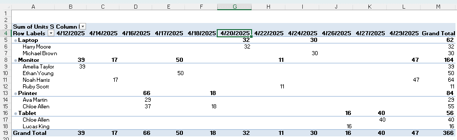
Step 3: Check the Pivot Table
This is not essentially a step; we are just going to analyze the pivot table to see the results. We have created a new column with the calculation using values from other columns.
➤ The pivot table has a lot of rows currently. If we go to the M4 cell, we can see that a new column has been added with the name “4th Week”.
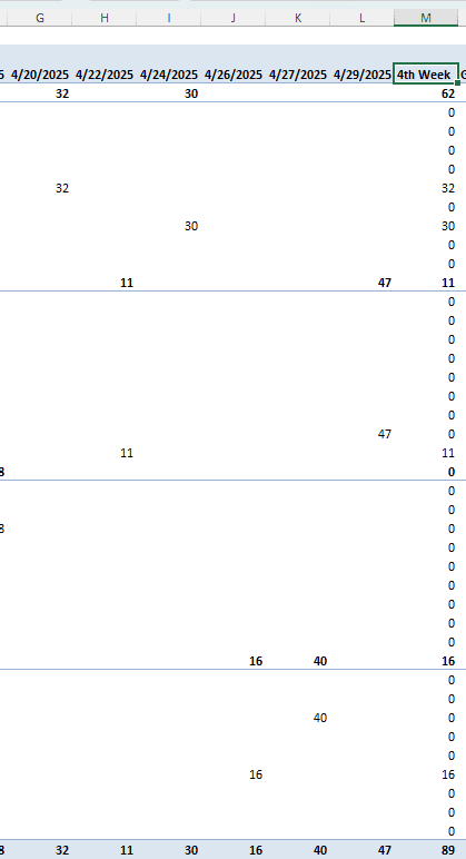
➤ This column is calculated by adding the values of 4/20/2025, 4/22/2025, 4/24/2025, and 4/26/2025.
Frequently Asked Questions
Can you create custom Calculations in a PivotTable?
There are two ways to do this. First, you can change the value calculations by right-clicking on a value and selecting “Summarizing Values By”. In the submenu, there will be a lot of calculation options like Sum, Count, Average, Max, Min, Product, etc. Secondly, you can create a calculated field by going to the PivotTable Analyze tab on the ribbon and selecting Calculations > Fields, Items, & Sets > Calculated Field. You can use custom formulas by this method, but no complicated functions can be used.
What is the difference between a calculated field and a calculated item in a PivotTable?
Calculated fields are used for a whole field. A field is a column header in the source dataset. A calculated field can do the calculations for the whole field from a formula. Calculated items, however, are similar to rows in the source dataset. It is more like adding a new row to the existing table, but by doing some calculations using the existing rows.
How to count distinct values in an Excel pivot table?
Distinct values cannot be counted in a pivot table without adding the pivot table to a data model. Create a new pivot table, and make sure that the option called “Add this data to the Data Model” is checked.
How can you refresh a PivotTable after updating the underlying data?
Pivot tables cannot be automatically refreshed after updating the underlying data. Instead, you have to do it manually. Right-click on the pivot table, and select Refresh to update the pivot table after you update the source dataset. You can also press Alt + F5 to refresh the pivot table, or go to the PivotTable Analyze column in the ribbon and select Refresh from the Data group.
Why can’t I use calculated fields in a PivotTable?
Because you have added the pivot table to a data model. Calculated fields and data models cannot coexist in a pivot table. Recreate the pivot table, and don’t add the table to a data model this time.
Wrapping Up
In this article, we have learned how to add a calculated field in a pivot table based on column values. Although it was not a perfect solution, it gets the job done, and that’s all you can ask for in this case. The Excel file we edited for this article can be downloaded for free. Feel free to use that to make the concept clearer.