
Renaming a column in Excel may sound simple, but it depends on what you’re working with. By default, the columns are named A, B, C, D and so on. Sometimes we may want to change their name to make them more meaningful and organized.
But Excel doesn’t allow us to change column names by default. So, most of us don’t know how to rename columns in excel and it seems to be a frustrating limitation. Fortunately, there are still some alternative options to change and display custom column names. Let’s walk through all the ways you can do it step by step.
➤ Click on the column header D.
➤ Go to the Display Bar on the top-right corner of the sheet.
➤ Click inside the bar and start typing the new name.
➤ Press Enter and we’re done.
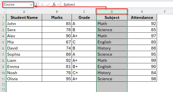
Rename Column for Basic Excel Worksheets from Display Bar
This would be the fastest method when you just need to change one or two headers. But it won’t be very effective when you work with larger worksheets and you want to rename many columns. Therefore, it won’t directly rename the column. We’ll just see the new name in the display bar once we click on the column.
For example, the worksheet we’ve below consists of five different columns naming A, B, C, and D. So, when we scroll down our column headings disappear and we can be distracted about the column name or what kind of information it has.

So, it’s a good idea to replace the columns A, B, C, and D with a proper name. To do so, we can simply rename each column the Display Bar and below we discuss how it works.
Steps:
➤ Locate the column header you want to change.
➤ Double click inside the Display Bar and remove the previous one or simply start typing the new name. The previous one will automatically be removed.
➤ Press Enter and now we can see that column A has been renamed to Name.
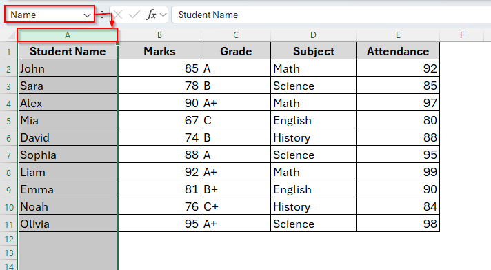
In the following image, we can see that if we click on column B, in the display bar, it shows B1.

Because we haven’t given it a name. Once we change the name like Column A, we’ll also see the new name in the display bar.
Rename Column Headers Using the Advance Option
The most effective way to rename a column in excel is using the Advance option. Unlike the previous method, it will completely replace the column headers A, B, C, and D with the names you require.
So, you don’t need to click on the column and locate the name in the display bar. You can see the column names in the first row.
Steps:
➤ Insert a new row in row 1. It will be our column header. So adjust it as you need, like give it a proper name, bold the font or change the background color for better visualization as we’ve done in the image below.

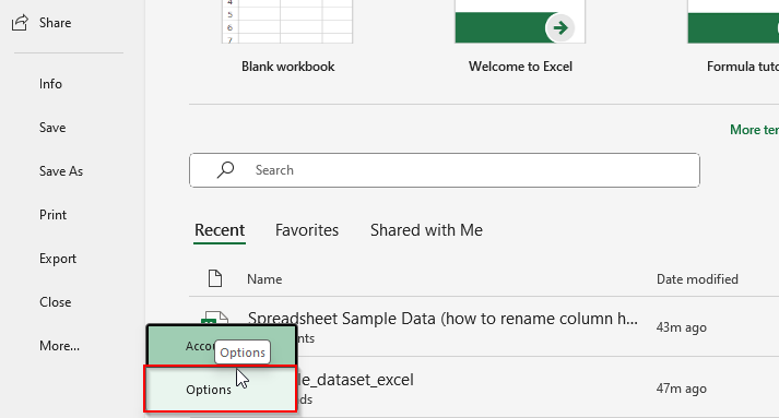
➤ Now go to File or just tap the Office button from the upper-left corner to locate the navigation pane. Choose Options from the lower-left corner of the navigation pane.
➤ Next select Advance and scroll down to locate Display options for this worksheet. Under this panel, uncheck the Show row and column headers box.
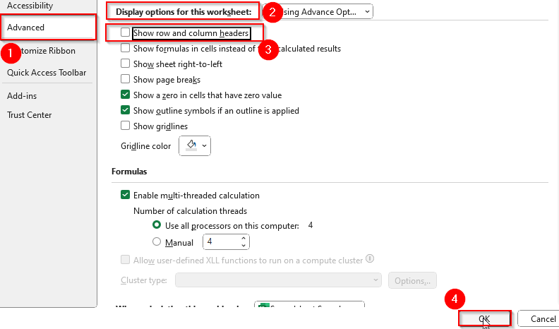
➤ By doing so, it will hide the default column headers and will only show the row you just created in the first step as column names.

But if you want to regain the default column headers, just navigate to Advance and check the Show row and column headers box again.
Renaming Column in an Excel Table
When you convert your data into an Excel Table, Excel treats headers differently. You can rename them directly in the table. It also allows you to do some automatic adjustments in the column name like sorting and filtering.
Therefore, if you update your dataset, for example, adding or removing new rows, it will still keep the column headers intact. So, it’s a very useful way to use tables while renaming a column name. Below are the steps to follow.
Steps:
➤ Create a new row in the beginning like the previous method.

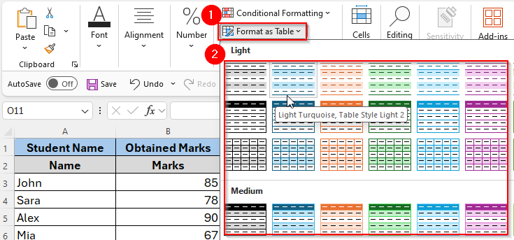
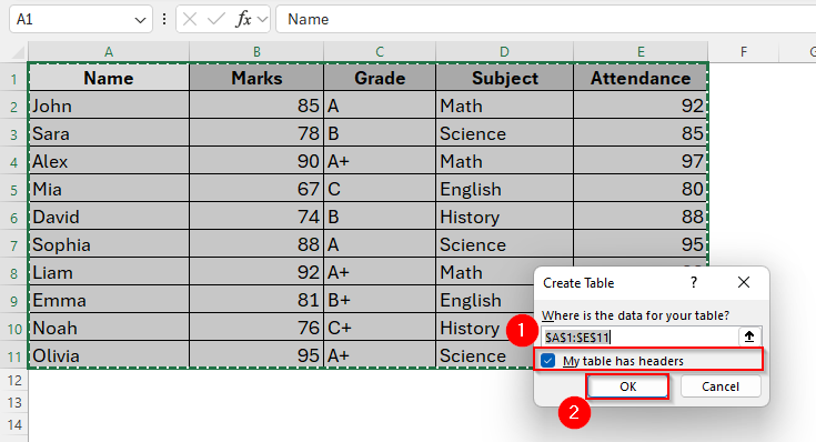
➤ Select the dataset and choose Format as Table. Alternatively, tap Ctrl + T from the keyboard. You’ll see many options to choose from for the specific table color. Choose whichever you like.
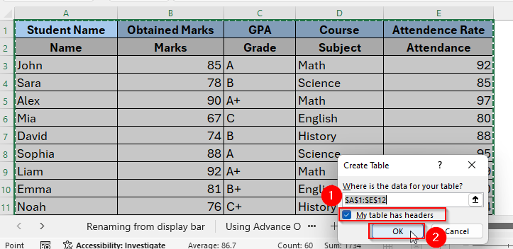
➤ Next make sure My table has headers box has been checked and press Ok.
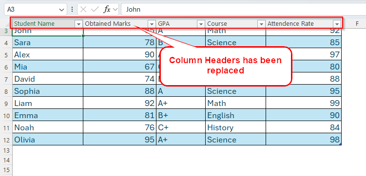
➤ Now your dataset has turned into a table and you can see the new column names in the first row. Most importantly, these names won’t disappear any more while you’re scrolling down to the sheet.
Renaming Column in Power Query
This is especially useful if you’re cleaning messy data or working with long datasets where consistent headers matter.
Steps:
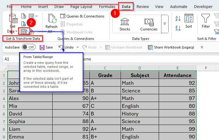
➤ Open the table in Power Query Editor. To do so, select your dataset and go to Data → From Table/Range from Get & Transform Data.
➤ Check the My table has headers box and click OK.
➤ Now our dataset has been transported to the Power Query Editor. So, just right-click any column header and select Rename.
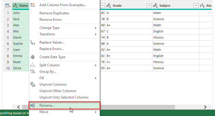
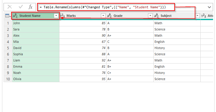
➤ Type the new name and press Enter. The column name has been replaced with the new name as the image shows below.
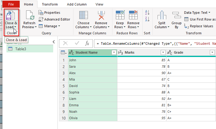
➤ Now click Close & Load to apply the change back into Excel.
Frequently Asked Questions (FAQs)
Will renaming a column affect my formulas?
If you’re using Excel Tables, formulas will automatically update to reflect the new column name. In normal worksheets, you may need to adjust formulas manually.
Can I use special characters in column names?
Yes, but it’s best to keep names simple like letters, numbers, and spaces. Avoid symbols that may confuse formulas.
Can I rename Excel’s built-in column letters (A, B, C…)?
No, Excel does not allow you to change those. You can only rename the headers by following some tricks as we discussed earlier.
Concluding Words
Renaming a column in Excel is one of those small but powerful steps that makes your data easier to read and work with. Whether you’re working in a basic worksheet, an Excel Table, or even Power Query, you have quick and simple options to update column headers. The key is to stay consistent with your names like clear headers mean fewer mistakes and smoother analysis.