Pivot Tables are one of the tools used in Excel for summarizing large datasets. By default, Pivot Tables provide a Sum as the subtotal for each group. However, for more versatile analysis, you might need different calculations like Average, Maximum, or Count. In this article, we will guide you through the process of creating custom subtotals in an Excel Pivot Table with some simple steps.
To create a custom subtotal in Excel Pivot Table, here is one simple solution by using the Field Setting feature.
➤ Select a cell from the column in which you want to create the custom subtotal.
➤ Right-click and select Field Settings from the context menu.
➤ In the Subtotals and Filters tab, choose Custom and select desired functions.
➤ Click OK, and your Pivot Table will show the selected subtotals for the chosen column.
Steps to Create Custom Subtotal in Excel Pivot Table
Here, we will create a Pivot Table from the dataset. Then we will apply the Field Settings feature to create custom subtotals. Adding numerous subtotals can make your PivotTable look cluttered. To fix this and make the data easy to read, we will format the Pivot Table.
Step 1: Creating Pivot Table with Sample Data
First, we will set up the Pivot Table using a sample dataset containing Store, Region, Product, and Monthly Sales data.
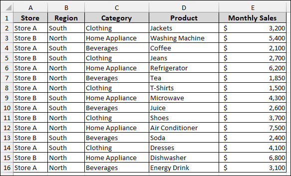
➤ Select your entire dataset, including the headers (cells A1 to E16).
➤ Go to the Insert tab and click on the PivotTable icon in the Tables group.

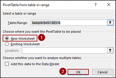
A dialog box will appear to define the Pivot Table parameters.
➤ In the dialog box, ensure the correct range is selected.
➤ Select New Worksheet to place the Pivot Table on a clean sheet.
➤ Click OK.
Next, we need to arrange the fields to create a structured report.
➤ In the PivotTable Fields pane, drag the Store, Region, and Product fields into the Rows area.
➤ Drag the Monthly Sales field into the Values area.
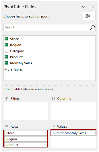
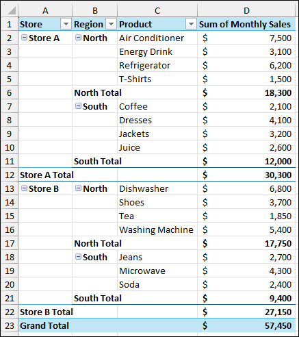
The resulting Pivot Table will display the Sum of monthly sales, with subtotals for the Region and Store groups. It shows the North Total and South Total within Store A and Store B, with an overall Grand Total.
Step 2: Using Field Settings Feature to Create Custom Subtotal
The default sum subtotal is often insufficient. We will now customize the subtotal for the Region field to include different calculations.
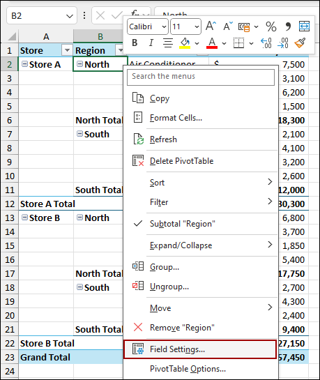
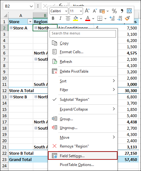
➤ Right-click on any cell containing a Region label (e.g., “North” in cell B2).
➤ From the context menu, select Field Settings.
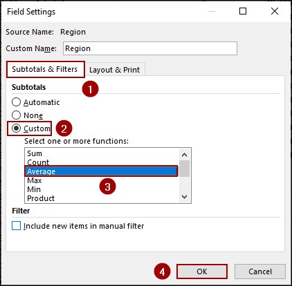
This opens the Field Settings dialog box.
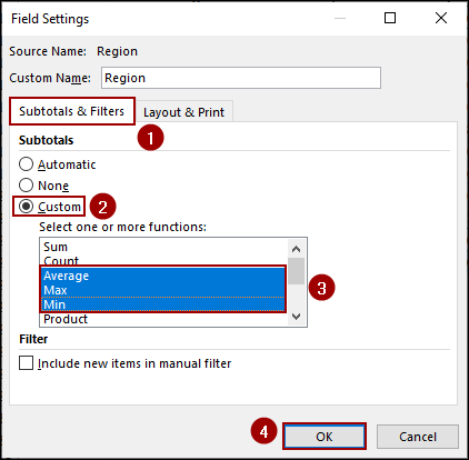
➤ In the Subtotals & Filters section, select the Custom option.
This reveals a list of Select one or more functions.
➤ Select the desired function.
We will choose Average to display the average sales for each region.
➤ Click OK.
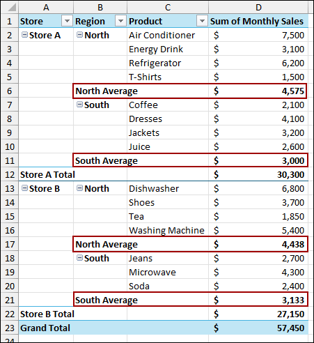
The Pivot Table will update, replacing the default North Total and South Total with North Average and South Average. Here, you will notice that the grand totals for the store remain, as we have included a subtotal for the Region column only.
You can also display multiple custom subtotals (e.g., Average, Max, and Min). For this,
➤ Right-click and choose Field Settings from the context menu.
➤ In the Field Settings dialog box, choose the Subtotals and Filters tab.
➤ Checkmark the Custom option and select multiple functions.
➤ After selecting, hit OK.
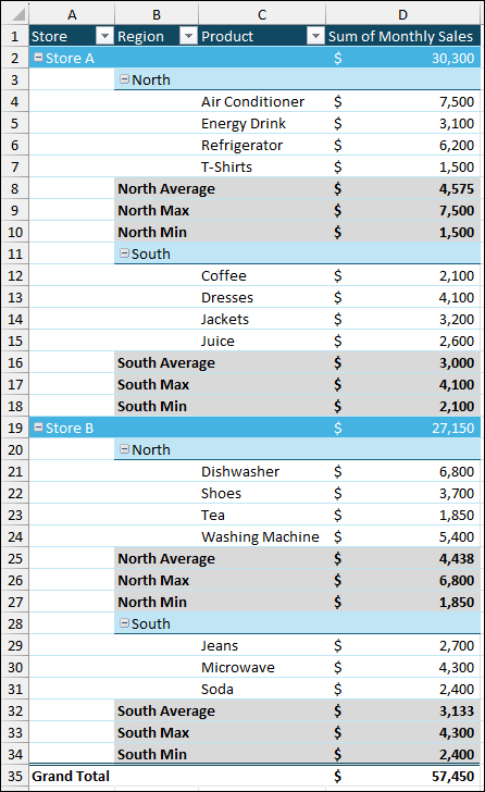
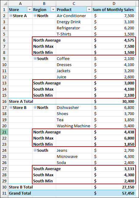
The Pivot Table will now show three separate subtotal rows for each region group: Average, Max, and Min of the Monthly Sales.
Step 3: Formatting Pivot Table
With multiple subtotals added, the Pivot Table can become hard to read. We can improve its readability using layout options and styling.
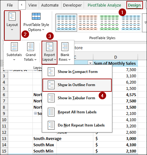
By default, Pivot Tables are displayed in Compact Form. Here, we will switch to Outline Form to get a better structure.
➤ Go to the Design tab on the ribbon.
➤ In the Layout group, click on Report Layout.
➤ Select Show in Outline Form.
This way, the Region and Product fields will move into their own dedicated columns.
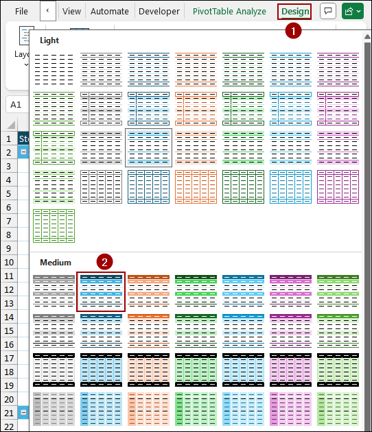
Finally, to give the Pivot Table a clean appearance, we will use one of Excel’s built-in styles.
➤ Click the Design tab.
➤ Select a style from the Medium section, such as the second blue option, to apply the formatting.
As a result, we will get a customized Pivot Table that provides Average, Max, and Min sales subtotals for each region, creating custom subtotals.

Frequently Asked Questions
Why are my custom subtotals not showing in the Pivot Table?
Custom subtotals may not appear if you have selected “Do not show subtotals” in the Design tab or you are using Tabular Form layout and have disabled subtotals.
Are custom subtotals available in all versions of Excel?
Custom subtotals are available in most modern versions, including Excel 2010, 2013, 2016, 2019, Excel 2021, and Microsoft 365. Some older versions may have limited subtotal options.
How do I reset a Pivot Table to default subtotals?
Go to PivotTable Analyze > Design > Subtotals > Show all Subtotals at Top/Bottom of Group, or select the field and click Field Settings > Automatic to restore default settings.
Concluding Words
Above, we have explored a step-by-step process to create custom subtotals in Excel Pivot Table. By utilizing the Field Settings feature and the Custom subtotal option, you can add multiple functions for the Pivot Table. This creation is important when the sum result does not provide a clear view. To get a complete overview of your Pivot Table, you need to add these subtotals. If you have any questions, please don’t hesitate to share them in the comments section below.