Excel’s built-in tool Solver is used for optimization. Solver is designed to find the best possible solution for complex decision-making problems, such as maximizing profit or minimizing costs. This entire process is known as linear programming. This technique is used for tasks like resource allocation, production planning, and scheduling in a business environment. In this article, we will provide a complete guide regarding the Excel Solver tool to solve a linear programming problem from start to finish.
To use the Solver for linear programming in Excel, here is one simple solution.
➤ Enable the Solver Add-in from File > Options > Add-ins > Excel Add-ins.
➤ Set up your objective function and constraints in the Excel sheet.
➤ Go to the Data tab and click Solver.
➤ Define the Objective, Variable Cells, and Constraints in the Solver Parameters dialog box.
➤ Select Simplex LP as the solving method.
➤ Click Solve to get the optimized value using Solver for linear programming.

What is Linear Programming?
Linear programming is a mathematical technique used to determine the best possible outcome (like maximum profit or lowest cost) in a model whose requirements are represented by linear relationships. Linear programming consists of three main components: Objective Function, Decision Variables, and Constraints. This is a fundamental concept in operations research and is widely applied in business for scheduling, production planning, and resource allocation.
Steps to Use Solver for Linear Programming in Excel
Here, we will use a step-by-step process to solve a linear programming problem using Excel Solver. We have broken down the process into three simple steps: preparing the model, enabling the Solver Add-in, and running the optimization.
Step 1: Preparing the Optimization Model
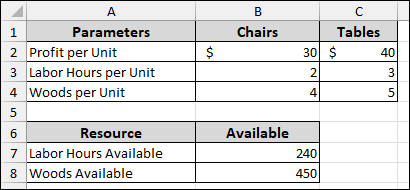
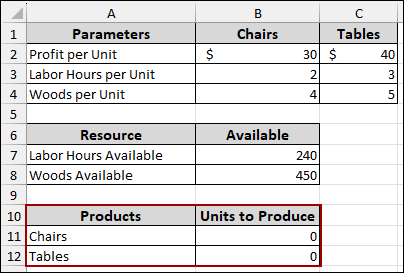
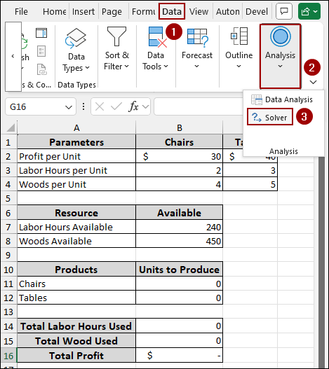
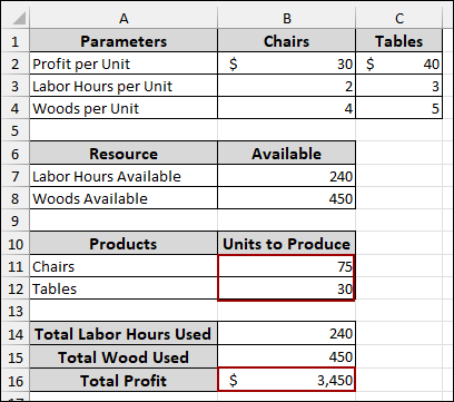
In this first step, we will organize our data and formulas in the Excel sheet to model a simple production planning problem. Our goal is to maximize the total profit from producing Chairs and Tables, limiting available labor hours and wood.
➤ First, set up a table listing the Parameters (Profit, Labor Hours, Wood) required per unit for both Chairs and Tables.
➤ Next, define the Resource section, showing the Available quantity for Labor Hours (240) and Wood (450).
This data represents our constraints.
➤ The cells next to these (B11 and B12) will be the Units to Produce (our decision variables), which the Solver will change.
➤ Enter a value of 0 in these cells.
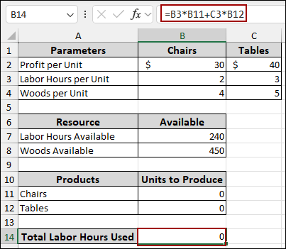
➤ In cell B14, enter the formula to calculate the Total Labor Hours Used.
=B3*B11+C3*B12
This multiplies the labor hours per unit by the units produced for both products and sums them up.
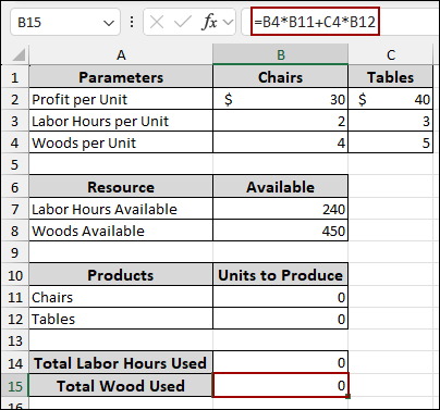
➤ Similarly, in cell B15, enter the formula to calculate the Total Wood Used.
=B4*B11+C4*B12
This represents the total wood consumed by the production plan.
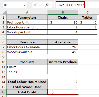
➤ In cell B16, write down the formula for the Total Profit.
=B2*B11+C2*B12
This formula calculates the total profit by multiplying the profit per unit by the units produced for each product.
The setup is now complete, with the objective function (Total Profit) and constraint formulas linked to the decision variables (Units to Produce).
Step 2: Enabling the Solver Add-in
Before running the optimization, you must ensure the Solver add-in is active in Excel.
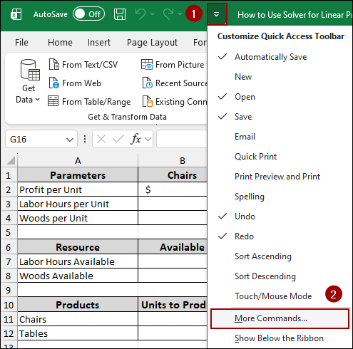
➤ Click the Customize Quick Access Toolbar dropdown arrow and select More Commands at the bottom of the list.
➤ In the Excel Options dialog box, click Add-ins on the left panel.
➤ From the Manage dropdown at the bottom, ensure Excel Add-ins is selected, and click Go.
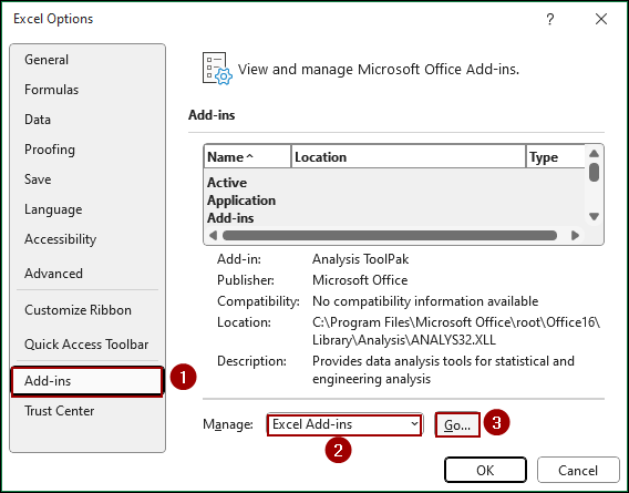
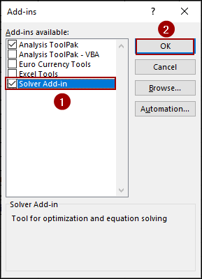
➤ In the Add-ins dialog box, checkmark the box next to Solver Add-in and click OK.
Once enabled, you will find the Solver button under the Data tab on the ribbon.
Step 3: Running the Optimization
With the model set up and Solver activated, we can now define the problem in the Solver tool.
➤ Go to the Data tab on the ribbon and click the Solver button within the Analysis group.
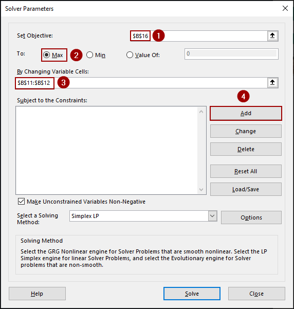
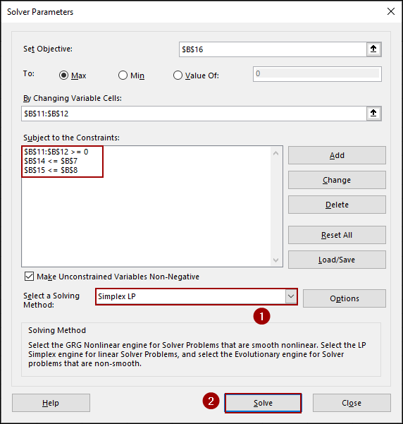
➤ In the Solver Parameters dialog box, set the Objective cell to $B$16 (Total Profit).
➤ Select Max to indicate we want to maximize the profit.
➤ Set the By Changing Variable Cells to $B$11:$B$12 (Units to Produce).
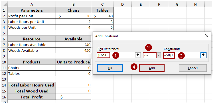
➤ Click the Add button to begin adding the constraints.
➤ For the Labor Hours constraint set Cell Reference to $B$14 (Labor Hours Used), select the constraint operator <=, and set the Constraint value to $B$7 (Labor Hours Available).
➤ Click Add.
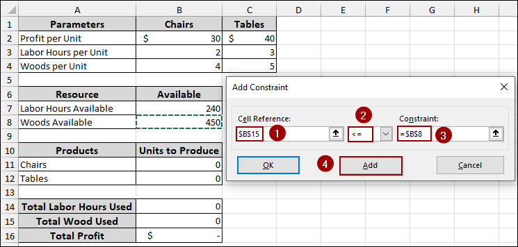
➤ For the Wood constraint set Cell Reference to $B$15 (Total Wood Used), select the constraint operator <=, and set the Constraint value to $B$8 (Wood Available).
➤ Hit Add.
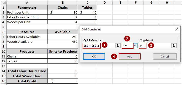
➤ For the non-negativity constraint (Units must be zero or positive), set Cell Reference to $B$11:$B$12 (Units to Produce), choose the constraint operator >=, set the Constraint value to 0.
➤ Press Add.
Back in the Solver Parameters dialog box, you will get all three constraints listed.
➤ In the Select a Solving Method dropdown, choose Simplex LP, as this is a linear programming problem.
➤ Click the Solve button.
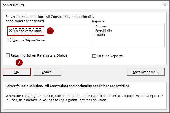
The Solver Results dialog box will appear.
➤ Select Keep Solver Solution and click OK.
The final result shows that by producing 75 Chairs and 30 Tables, the company maximizes its Total Profit at $3,450, using exactly 240 labor hours and 450 wood units. This way, you can use Solver for linear programming in Excel.
Frequently Asked Questions
Can I use Solver for non-linear problems?
Yes. While the Simplex LP method is for linear problems, Solver also offers the GRG Nonlinear for smooth nonlinear problems and the Evolutionary method for non-smooth problems.
What does it mean if Solver finds ‘no feasible solution’?
This means your constraints are too restrictive. For example, if the required resources for production exceed the available resources, no valid solution can be found. You would need to change one or more constraints and re-run Solver.
What is the difference between Simplex LP and GRG Nonlinear?
Simplex LP is exclusively for optimization problems where all relationships (objective and constraints) are linear, providing an optimal solution. GRG Nonlinear is used when the relationships are curved or non-linear, but it can only find a simple optimal solution.
Concluding Words
Above, we have covered all the steps to use Solver to find the optimal solution for a linear programming problem. By properly defining your objective, decision variables, and constraints, you can solve any complex task. While inserting constraints, make sure to provide all the conditions of your problem. If you have any questions, please don’t hesitate to share them in the comments section below.