The Sum of Years’ Digits depreciation method is used in corporations that favor having a larger depreciation in the earlier years of the asset’s life. Most assets lose value quickly at the beginning, as even if you are selling a one-day used product, you will get a lot lower price than you paid for it. You will have to pay less tax in the earlier years of the asset’s life as well because of higher depreciation. In this article, we will learn the sum of years’ digits depreciation formula in Excel.
➤ Use the following formula to calculate the depreciation:
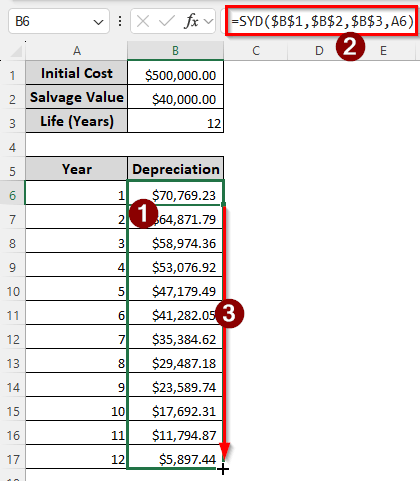
=SYD($B$1,$B$2,$B$3,A6)
➤ Replace $B$1 with the initial cost of the asset, $B$2 with the salvage value, $B$3 with the life of the asset, and A6 with the current year.
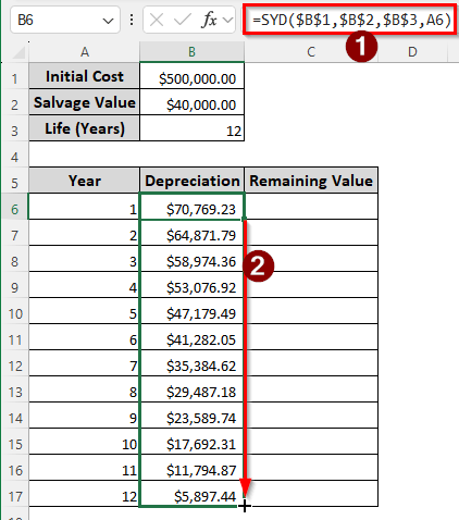
➤ Drag the autofill handler to fill up the depreciation table.
In this article, we will learn what the sum of years’ digits depreciation method is, and what formulas we can use to calculate it in Excel. Download the Excel file provided with this article to see the methods we use in action by yourself. Let’s begin.
What is the Sum of Years’ Digits Depreciation Method?
In general, depreciation is the method of distributing the cost of an asset between multiple years so that the business can prepare when it eventually has to replace the asset. In the sum of years’ digits depreciation method, we measure the percentage of depreciation by dividing the sum of years by the remaining years left on the life of the asset. Then, we multiply it by the depreciation basis (cost of the asset – salvage value) to calculate the depreciation.
Using the SYD Function to Calculate the Depreciation in Excel
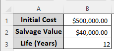
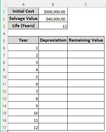
Here, we have the initial cost of the asset, the salvage value, and the life of the asset. The easiest way to calculate the depreciation using these three pieces of information is using the SYD function provided by Microsoft Excel itself. Here is how to do it:
➤ Create a table with the following columns:
Year, Depreciation, Remaining Value.
➤ Fill up the Year column with a 1-12 year count.
➤ In the B6 cell, insert the following formula, and autofill the column:
=SYD($B$1,$B$2,$B$3,A6)
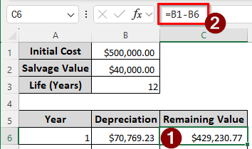
➤ In the C6 cell, calculate the initial value of the first year using the formula below:
=B1-B6
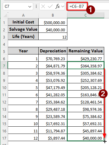
➤ Use the following formula in the C7 cell, and autofill till C17:
=C6-B7
Calculating the Sum of Years’ Digits Depreciation Manually
Instead of using the dedicated function provided by Excel, we can calculate the depreciation using a manual formula as well. Follow the instructions below to do it:
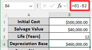
➤ Measure the depreciation base using the following formula in the B4 cell:
=B1-B2
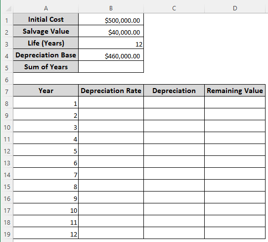
➤ Create a table for the depreciation schedule with the following columns:
Year, Depreciation Rate, Depreciation, Remaining Value.
➤ Fill up the Year column with the years for 1-12, like the previous method.
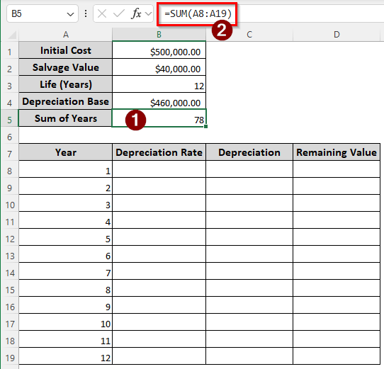
➤ Calculate the sum of years in the B5 cell using the following formula:
=SUM(A8:A19)
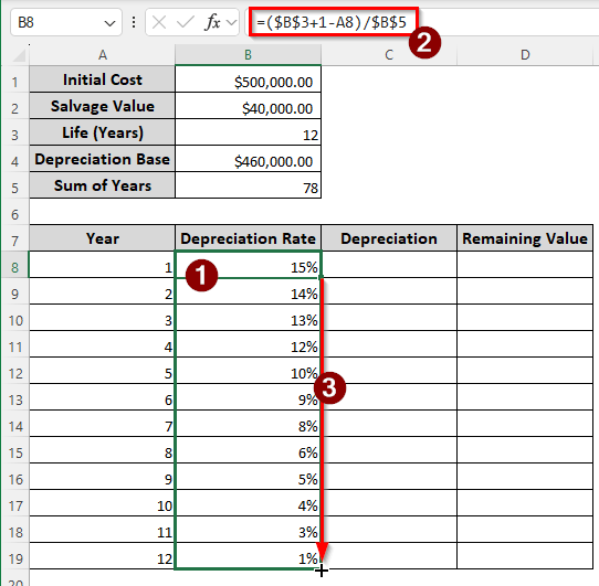
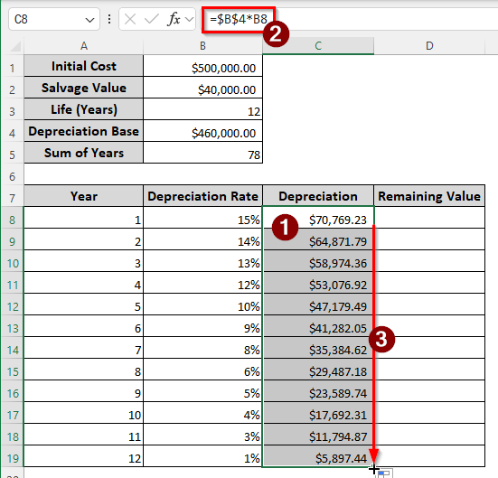
➤ Calculate the depreciation rate in the B8 cell using the following formula, and autofill the column:
=($B$3+1-A8)/$B$5
➤ Calculate the depreciation using the following formula in the C8 cell:
=$B$4*B8
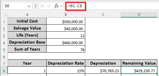
➤ Calculate the first remaining value with the formula below:
=B1-C8
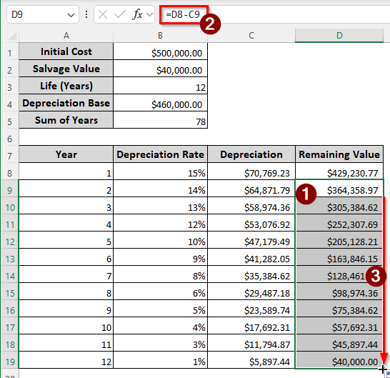
➤ The following formula should be put in the D9 cell, and the rest of the rows till D19 should be autofilled for the rest of the remaining values:
=D8-C9
Frequently Asked Questions
What is the formula for the sum of years’ digits of depreciation?
For manual calculation, the formula for the sum of years’ digits depreciation is as follows:
Depreciation=(Remaining Useful Life/Sum of Years’ Digits) * Depreciable Basis
How to calculate the sum of digits in Excel?
You can use the SUM functions to do that. Here is the potential formula for that:
=SUM(A1:A10)
Here, A1:A10 is the range of the cells that contain the digits.
How to calculate years of depreciation?
How many years you will calculate the depreciation for depends on your company and its accounting principles. There is no fixed formula or rule for the number of years of depreciation, and thus, it cannot be calculated.
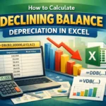
What is the formula for depreciation in Excel?
There are five dedicated functions for depreciation in Excel. Those are SLN, SYD, DB, DDB, and VDB. All of them require the cost of the asset, the salvage value of the asset, and the lifetime of the asset. SYD, DB, and DDB require the current year for which the depreciation is calculated, and VDB requires the starting and ending period of depreciation.
How to calculate digits in Excel?
To calculate how many digits there are in a cell, use the following formula:
=LEN(A1)
Here, replace the cell of A1 to calculate the digits of.
Wrapping Up
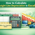
We have learned how to calculate depreciation using the sum of years’ digits depreciation method. The tutorial has shown two methods, one with the manual formula and one with the dedicated function provided by Excel. Should you have any questions, leave them in the comment section, and we will get back to you. See you in the next article.