Finding duplicate rows based on multiple columns in Excel helps you clean and organize data accurately. It ensures that each unique record appears only once, especially when the same combination of values repeats across multiple columns. For example, two records may share the same Customer ID, Product ID, and Order Date, which means they represent the same transaction entered more than once.
In this article, you’ll learn how to find duplicate rows based on multiple columns in Excel step by step using several easy methods.
Here’s how to find duplicate rows based on multiple columns in Excel:
➤ Open your dataset in Excel. Add a helper column in column E and label it Combined Key.
➤ Click on cell E2 and enter the following formula:
=A2 & ” | ” & B2 & ” | ” & TEXT(C2,”yyyy-mm-dd”)
➤ Press Enter. You’ll now see a combined value in cell E2.
➤ Drag the fill handle down to apply the formula to the rest of the rows in column E.
➤ Add a new column in column F and label it Duplicate Status.
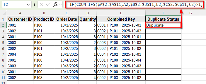
➤ In cell F2, enter this formula:
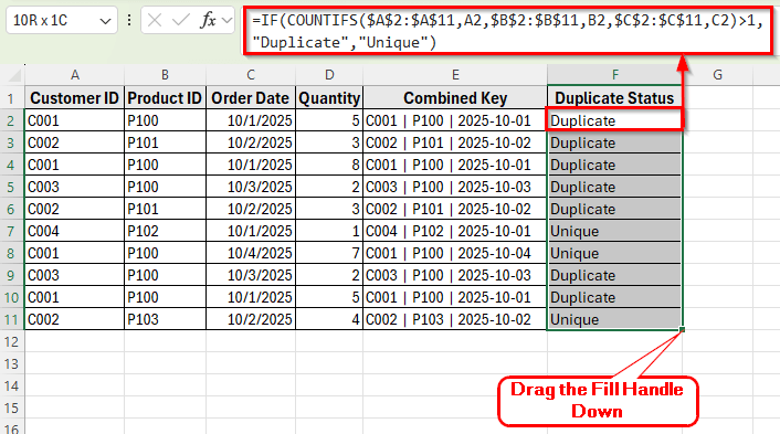
=IF(COUNTIFS($A$2:$A$11,A2,$B$2:$B$11,B2,$C$2:$C$11,C2)>1,“Duplicate”,”Unique”)
➤ Press Enter. Excel will show Duplicate if the same combination appears more than once, or Unique if it’s the only one of its kind.
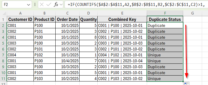
➤ Drag the fill handle down to apply the formula to the rest of the rows in column F.
Using Helper Column and COUNTIFS to Find Duplicate Rows
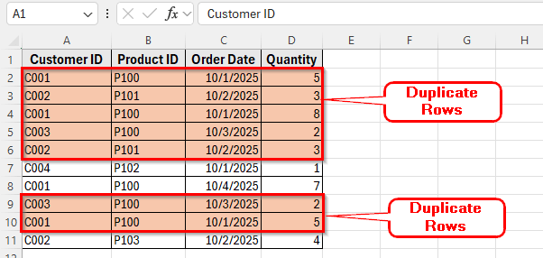
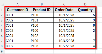
In the following dataset, we have a small list of transactions. Column A lists Customer ID, Column B lists Product ID, Column C lists Order Date, and Column D lists Quantity.
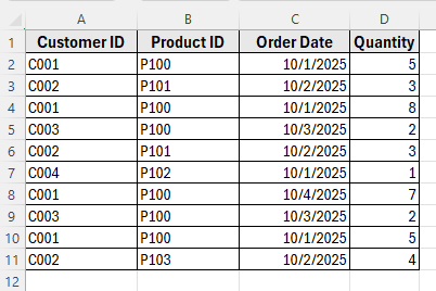
We’ll use this dataset to demonstrate how to find duplicate rows based on columns A, B and C.
The COUNTIFS function is one of the most effective ways to find duplicate rows based on multiple columns in Excel. It counts how many times a specific combination of values appears across selected columns. If the count is greater than 1, that means the row is a duplicate.
This method is helpful when you want to clearly mark duplicates instead of removing them.
Here’s how to do it step by step:
➤ Open your dataset in Excel. Add a helper column in column E and label it Combined Key, where you want to combine the values of the key columns such as Customer ID, Product ID, and Order Date.
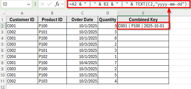
➤ Click on cell E2 and enter the following formula:
=A2 & " | " & B2 & " | " & TEXT(C2,"yyyy-mm-dd")
➤ This formula joins the three columns into one text string for easy comparison.
➤ Press Enter. You’ll now see a combined value in cell E2.
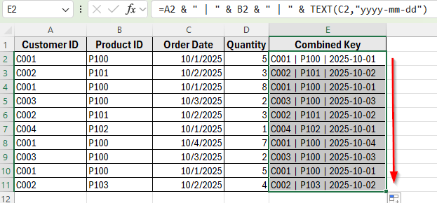
➤ Drag the fill handle down to apply the formula to the rest of the rows in column E. Now that all rows are combined, we can check how many times each combination appears.
➤ Add a new column in column F and label it Duplicate Status, where you want to show whether each row is marked as Duplicate or Unique.
➤ In cell F2, enter this formula:
=IF(COUNTIFS($A$2:$A$11,A2,$B$2:$B$11,B2,$C$2:$C$11,C2)>1,"Duplicate","Unique")
➤ Press Enter. Excel will show Duplicate if the same combination appears more than once, or Unique if it’s the only one of its kind.
➤ Drag the fill handle down to apply the formula to the rest of the rows in column F.
Highlight Duplicate Rows Using Conditional Formatting
If you want to visually highlight duplicate rows instead of tagging them with text, you can use Conditional Formatting with a custom COUNTIFS formula. This method is ideal when you need to quickly see which rows are duplicated based on multiple columns.
Here’s how to do it step by step:
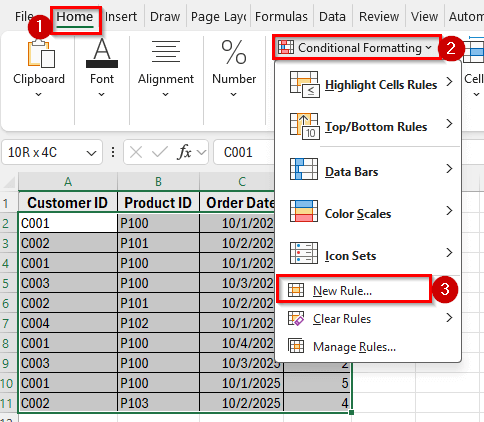
➤ Select the range A2:D11, which includes all your data without the headers.
➤ Go to the Home tab on the Excel ribbon, click Conditional Formatting, then choose New Rule.
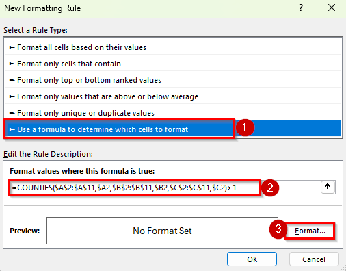
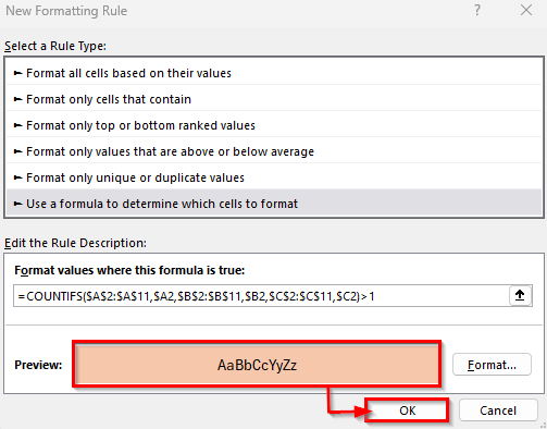
➤ In the New Formatting Rule window, select Use a formula to determine which cells to format.
➤ In the formula box, enter this formula:
=COUNTIFS($A$2:$A$11,$A2,$B$2:$B$11,$B2,$C$2:$C$11,$C2)>1
➤ This formula checks each row and highlights it if the combination of Customer ID, Product ID, and Order Date appears more than once in the dataset.
➤ Click Format.
➤ In Format Cells window, choose a fill color such as light red, and then click OK.
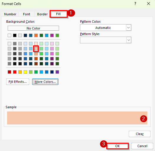
➤ Click OK again to apply the rule.
➤ Now Excel will highlight all rows that have duplicate combinations across the selected columns.
Find and Clean Duplicate Rows Using the Remove Duplicates Tool
Excel’s built-in Remove Duplicates feature is a simple and effective way to find and remove duplicate rows based on multiple columns. It quickly scans the selected columns and removes rows that share the same combination of values. This method works best when you want to keep only one instance of each unique record.
Here’s how to do it:
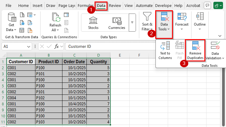
➤ Select the range A1:D11, including the headers.
➤ Go to the Data tab on the Excel ribbon and click Remove Duplicates in the Data Tools group.
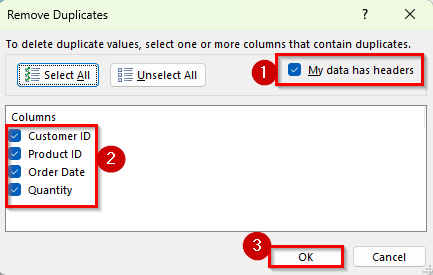
➤ A dialog box will appear. Make sure the option My data has headers is checked.
➤ In the list of columns, select Customer ID, Product ID, and Order Date because these are the columns you want to check for duplicates.
➤ Click OK. Excel will now search for rows where the combination of these three columns is repeated. It will keep the first occurrence and remove all other duplicates.
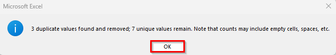
➤ A confirmation message will appear showing how many duplicate rows were removed and how many unique values remain.
➤ Click OK.
➤ Now you will get clean and unique values in your dataset.
Note:
Before using this tool, it’s a good idea to make a backup of your worksheet since the duplicates are deleted instantly.
Using Advanced Formulas to Identify Complex Duplicate Rows
In some cases, you may need more flexible or dynamic ways to find duplicates, especially in large datasets or when you want to display only the duplicate rows. For these situations, advanced formulas like UNIQUE, FILTER, and COUNTIFS together can help. These formulas are available in modern Excel versions such as Excel 365 and Excel 2021.
Here’s how to do it step by step:
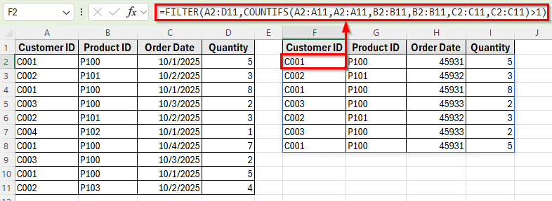
➤ Click on an empty cell, such as F2, and enter the following formula:
=FILTER(A2:D11,COUNTIFS(A2:A11,A2:A11,B2:B11,B2:B11,C2:C11,C2:C11)>1)
➤ This formula filters and displays only the rows that have duplicates across the selected columns such as Customer ID, Product ID, and Order Date.
➤ Press Enter. Excel will instantly show only the duplicate rows from your dataset in a new range.
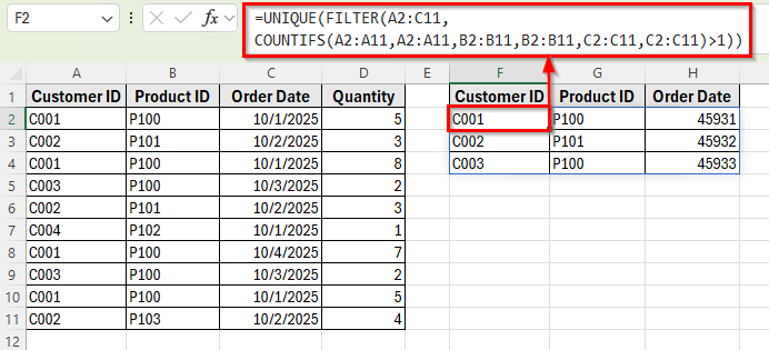
➤ If you only want to list unique duplicate combinations without repeating them multiple times, use this version:
=UNIQUE(FILTER(A2:C11,COUNTIFS(A2:A11,A2:A11,B2:B11,B2:B11,C2:C11,C2:C11)>1))
➤ This will return each duplicated combination once.
Frequently Asked Questions
How can I find duplicates based on only two columns instead of three?
You can simply adjust the formula or the Remove Duplicates selection. For example, use this formula if you only want to compare Customer ID and Product ID:
=COUNTIFS($A$2:$A$11,A2,$B$2:$B$11,B2)>1
This will flag any rows that share the same Customer ID and Product ID combination.
What if I want to find duplicates without deleting them?
You can use either the COUNTIFS formula or Conditional Formatting methods. Both will identify duplicates without removing any data, allowing you to review them first.
Can I remove duplicates and keep the first occurrence?
Yes. The Remove Duplicates tool automatically keeps the first instance of each combination and deletes the rest. Before doing this, it’s best to make a copy of your data as a backup.
Wrapping Up
Finding duplicate rows based on multiple columns in Excel becomes necessary when you work with large datasets that may include repeated entries. It helps maintain data integrity by ensuring that each record is unique and accurate.
This process is especially useful for cleaning reports, consolidating data from multiple sources, and preparing datasets for analysis.
By identifying and managing duplicates, you can prevent calculation errors, avoid misleading summaries, and keep your data well-organized.