Counting colored cells in Excel helps you analyze data visually marked with highlights, such as completed tasks, sales regions, or product categories. Excel doesn’t have a built-in formula to count by color, but there are easy ways to do it without writing VBA code.
In this article, you’ll learn how to count colored cells in Excel without VBA, using different methods.
Here’s how to count colored cells in Excel without VBA:
➤ Go to the Formulas tab and click Name Manager >> New.
➤ In the New Name window enter a name like COLOREDCELLS.
➤ In the Refers to box, type this formula: =GET.CELL(38,Sheet1!C2)
➤ Click OK to save.
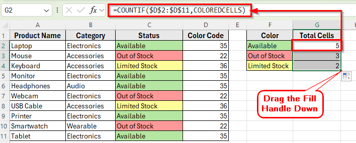
➤ In cell D2, type this formula to get the color index: =COLOREDCELLS
➤ Then drag the fill handle down to apply it for all rows.
➤ Next, create a result table in Column F and Column G. Label them Color and Total Cells.
➤ Under the Color column, type the unique status name with filled color you used in the Status column
➤ To count cells with a specific color, type this following formula in cell G2:
=COUNTIF($D$2:$D$11,COLOREDCELLS)
➤ This gives you the exact count of cells matching that color.
➤ Then drag the fill handle down to apply it for the rest of the rows.
Count Colored Cells Using Filter and SUBTOTAL in Excel
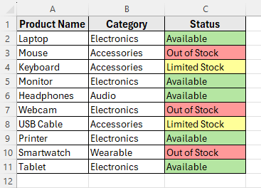
In the following dataset, we have a list of Products along with their Category and Status. The Status column is color-coded such as Green for Available, Yellow for Limited Stock, and Red for Out of Stock.
We’ll use this dataset to count these colored cells using simple, no-VBA methods.
This is the easiest way to count colored cells in Excel without using any VBA code. You can filter your dataset based on cell color and then apply the SUBTOTAL function to count only the visible cells.
Here’s how to do it step by step:
➤ Open your dataset in Excel.
➤ Select any cell inside your data range.
➤ Go to the Data tab on the ribbon and click Filter.
➤ This adds filter drop-down arrows beside each header in your dataset.
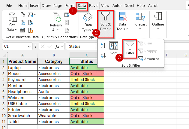
➤ Click the arrow next to the Status column header.
➤ From the drop-down list, choose Filter by Color and select the color you want to count. For example, select Green, which represents Available items.
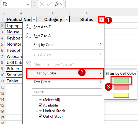
➤ After applying the filter, Excel will display only the rows containing the selected color. All other rows will be hidden temporarily.
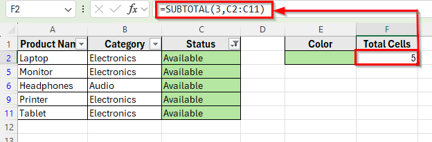
➤ Now, select a blank cell below your table where you want to display the count.
➤ Type the following formula:
=SUBTOTAL(3,C2:C11)
➤ Press Enter to get the result.
➤ Excel will now return the count of colored cells that are currently visible after applying the filter.
➤ For example, if you filtered by the Green color, and 5 cells are Green, the result will show 5.
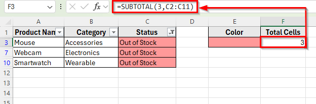
➤ To count another color, clear the filter and repeat the same steps for Red.
Using Find and Replace Tool to Count Colored Cells in Excel
This method works well if you just want to quickly see how many cells share the same color, without formulas.
Here’s how to do it:
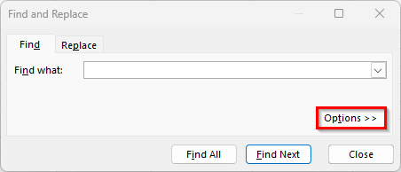
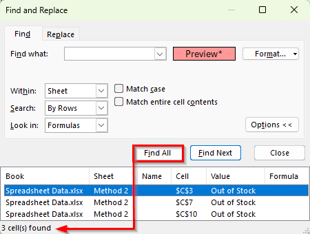
➤ Go to the Home tab and click Editing >> Find & Select >> Replace or simply press Ctrl + F in your keyboard to open the Find and Replace dialog box.
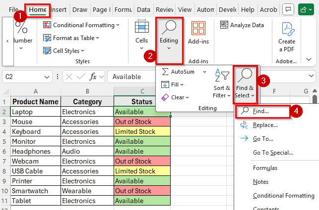
➤ Click Options to expand more settings.
➤ Click Format >> Choose Format From Cell.
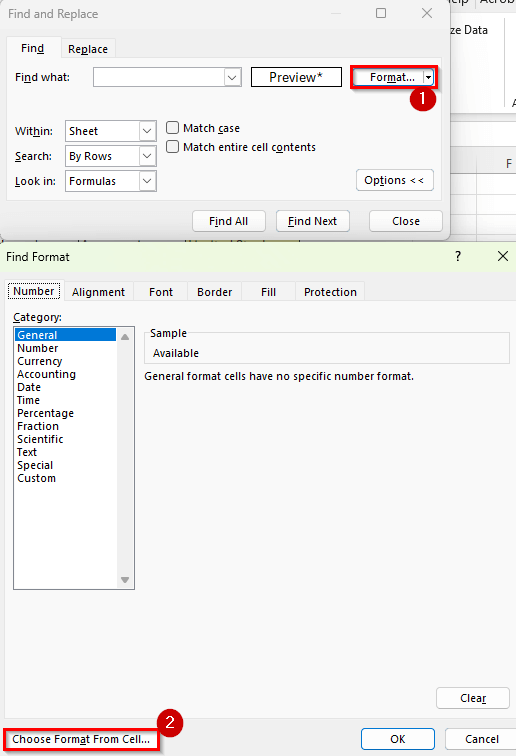
➤ Now click on a cell with the fill color you want to count. For example, Green.
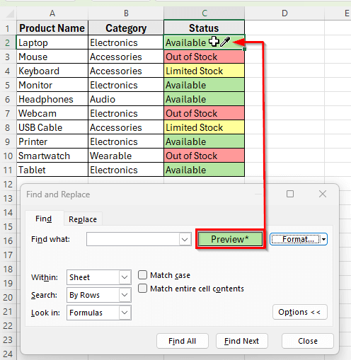
➤ After selecting the color, click Find All.
➤ At the bottom of the window, Excel will list all cells that match that fill color.
➤ Check the bottom-left corner. You’ll see 5 cells found, showing the count instantly.
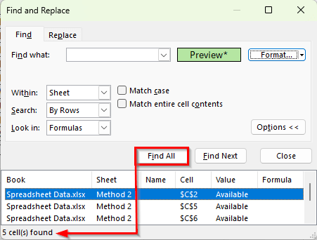
➤ To find another color, follow the same steps and choose the format Red.
Count Colored Cells Using GET.CELL Function via Named Range
Excel’s GET.CELL is an old but useful function that can detect the color index of a cell. You can combine it with COUNTIF to count colored cells without VBA.
Here’s how to do it step by step:
➤ Go to the Formulas tab and click Defined Names >> Name Manager.
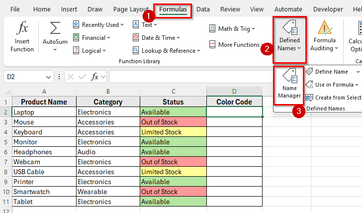
➤ Click New.
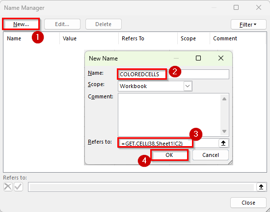
➤ In the New Name window enter a name like COLOREDCELLS.
➤ In the Refers to box, type this formula:
=GET.CELL(38,Sheet1!C2)
➤ Here 38 returns the color index code of the cell C2.
➤ Click OK to save.
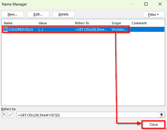
➤ Click Close to close the Name Manager window.
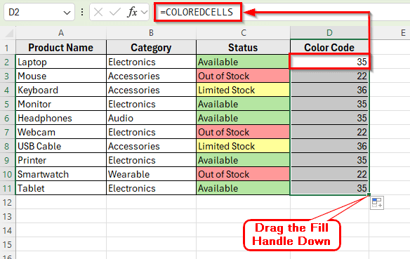
➤ In cell D2, type this formula to get the color index:
=COLOREDCELLS
➤ Then drag the fill handle down to apply it for all rows.
➤ You’ll now see numbers like 35, 22, 36, etc., representing the color index of each cell.
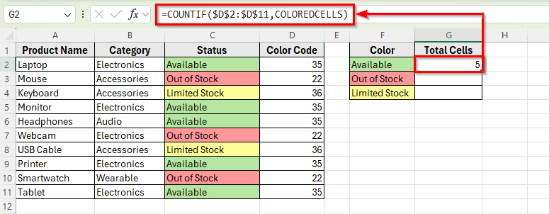
➤ Next, create a result table in Column F and Column G. Label them Color and Total Cells.
➤ Under the Color column, type the unique status name with filled color you used in the Status column
➤ To count cells with a specific color, type this following formula in cell G2:
=COUNTIF($D$2:$D$11,COLOREDCELLS)
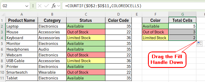
➤ This gives you the exact count of cells matching that color.
➤ Then drag the fill handle down to apply it for the rest of the rows.
Frequently Asked Questions
How can I count colored cells automatically in Excel?
You can use the GET.CELL formula through a Named Range and then combine it with COUNTIF. This method automatically updates counts when colors change after recalculating (press F9).
Can I use COUNTIF directly to count colored cells?
No. COUNTIF can’t recognize cell color. You need a helper column like one created with GET.CELL, that stores the color code first.
Why doesn’t Excel have a built-in function to count by color?
Because colors are formatting attributes, not cell values. Excel formulas calculate based on data, not appearance.
Wrapping Up
Counting colored cells in Excel is helpful when your data uses highlights to represent specific categories or progress levels. It helps you analyze visual information, such as tracking completed tasks, checking available products, or identifying delayed projects.
By counting based on color, you can quickly summarize your dataset without reading every entry. It saves time and gives a clearer view of the overall status in your worksheet.