Working with name lists in Excel can sometimes be a hassle, especially when the names are in the wrong order. Maybe you’re sorting a customer database, formatting survey responses, or preparing a mailing list. If your names are listed as “Last, First” and you need them in the “First Last” format or the other way around, Excel doesn’t have a direct button for that.
But don’t worry. With just a few easy-to-follow steps, you can reverse names using built-in Excel functions like LEFT, RIGHT, FIND, and MID. These formulas make it simple to clean up your data and reformat names exactly how you need them, no special tools or add-ons required.
In this article, we’ll walk you through several effective methods, complete with clear examples and step-by-step instructions, so you can choose the best solution for your task.
Steps to reverse names using TEXT function:
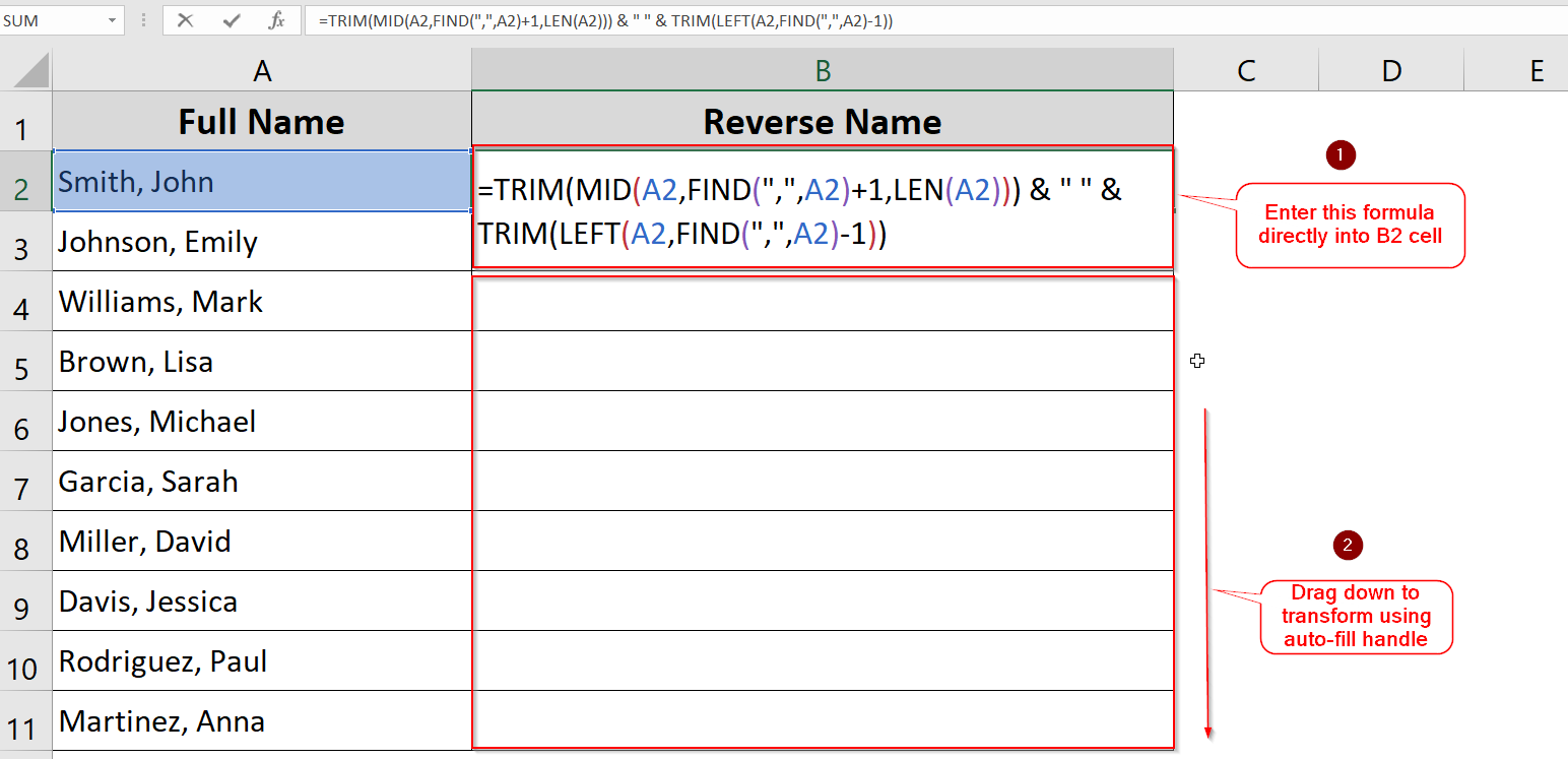
➤ Paste formula in B2 cell:
=TRIM(MID(A2,FIND(“,”,A2)+1,LEN(A2))) & ” ” & TRIM(LEFT(A2,FIND(“,”,A2)-1))
➤ Click Enter.
➤ Drag down to apply to all cells.
What is “Reverse Names” in Excel?
Reversing names in Excel means changing the order in which parts of a name appear. For example, if a name is written as “Doe, Jane”, you might want it to display as “Jane Doe” instead. This is a common task when working with data from various sources like CRMs, sign-up forms, or databases, where the name format might not be consistent.
Reordering names ensures everything follows the same structure, which is especially useful for sorting lists, preparing reports, or creating mailing labels. Excel offers several simple methods to reverse name order, including formulas, Flash Fill, and the Text to Columns tool.
Apply Text Functions to Reverse “Last, First” Format
When names are entered in the “Last, First” format it can make sorting, filtering, or mail merging a bit messy. Thankfully, Excel lets you reverse this format using a simple formula that rearranges the names into a more natural “First Last” format.
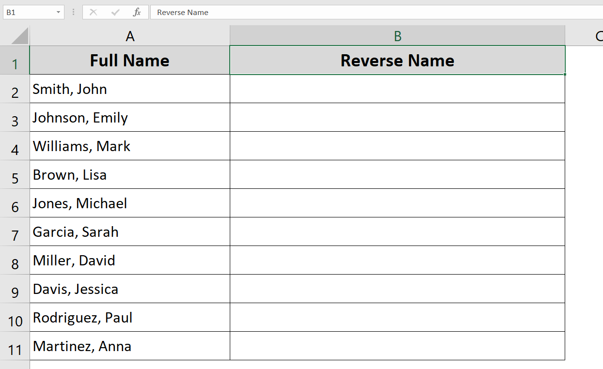
In our example dataset, the original names are listed under the Full Name column (Column A). We’ll use a formula in the adjacent Reversed Names column (Column B) to automatically flip each name from “Last, First” to “First Last”.
This method is ideal for cleaning up contact lists, spreadsheets for email marketing, or any Excel file where consistent name formatting matters.
Steps:
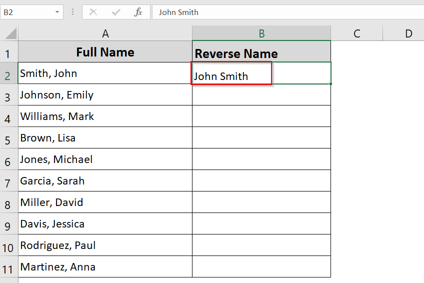
➤ In cell B2, enter the following formula:
=TRIM(MID(A2,FIND(“,”,A2)+1,LEN(A2))) & ” ” & TRIM(LEFT(A2,FIND(“,”,A2)-1))
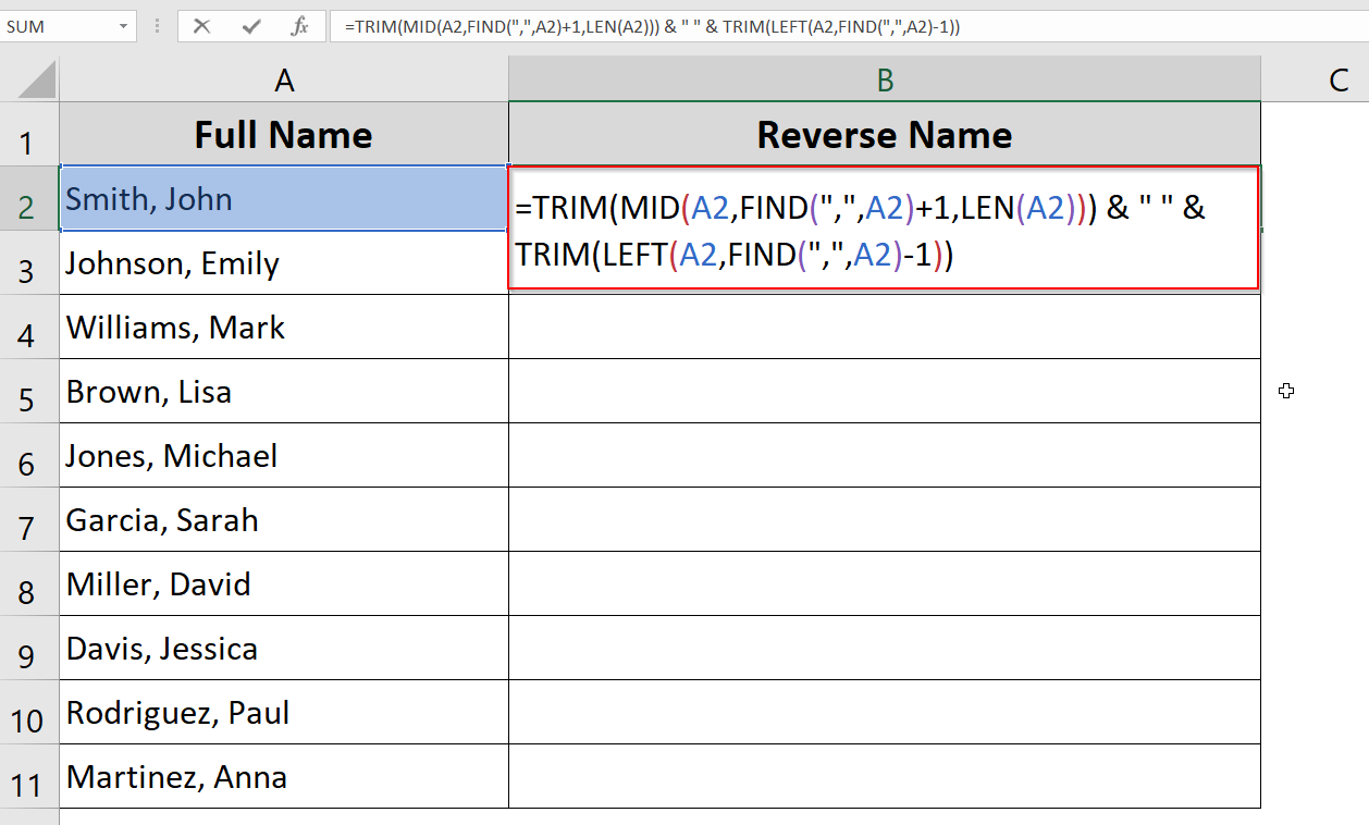
➤ Press Enter and drag the fill handle down to apply it to the other cells.
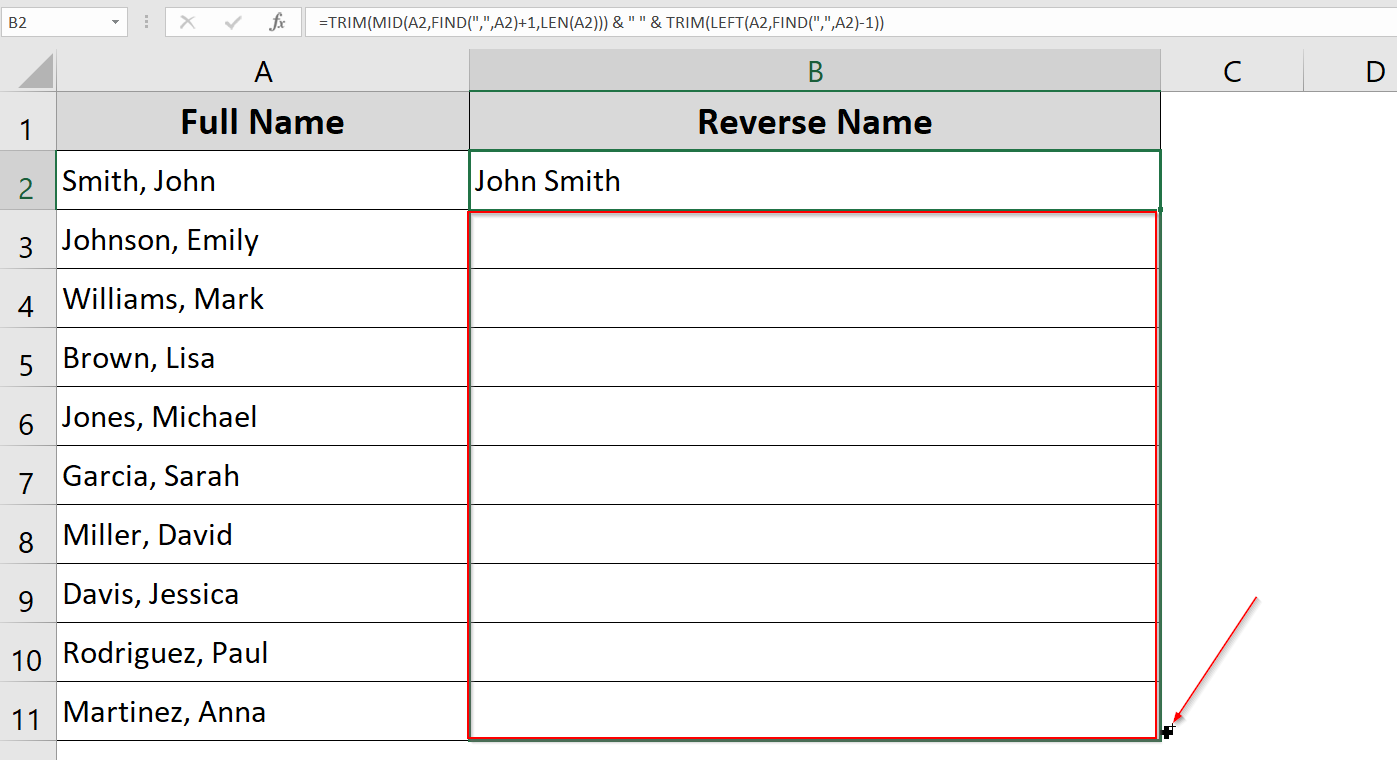
This will convert “Smith, John” into “John Smith” while removing extra spaces.
Use Flash Fill (Excel 2013 and later)
Flash Fill can save you tons of time. It’s a smart tool that recognizes patterns in your data and automatically completes the rest of the column for you, without the need for complex formulas or extra functions.
Flash Fill is perfect for reversing names because it learns from your example. For instance, if you have a list formatted as “Brown, Lisa” and want it to appear as “Lisa Brown”, all you need to do is manually type the first name correctly in the adjacent column. Once Excel picks up the pattern, it will automatically suggest the rest.
Steps:
➤ In cell B2, type the reversed version of the first name (e.g., “John Smith”).
➤ Press Enter.
➤ In cell B3, start typing the next reversed name. Excel will detect the pattern and preview the rest.
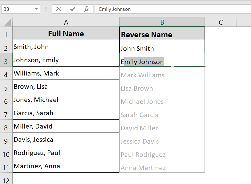
➤ Press Enter again to accept the Flash Fill suggestions.
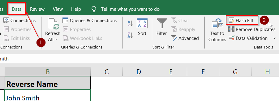
➤ If Flash Fill doesn’t auto-trigger, go to Data >> Flash Fill or press Ctrl + E.
Try Text to Columns Feature & Then Concatenate
If your names are separated by a comma, this method is a great way to split and reorder them. It’s a visual, hands-on approach that works well for people who prefer not to use complex formulas.
Excel’s Text to Columns tool helps you break the name into separate parts, and then you can use a simple formula like CONCATENATE or TEXTJOIN to rearrange the pieces in the order you want. This method is especially useful for short lists where accuracy and control matter.
Steps:
➤ Select the column with the names (e.g., A2:A11).
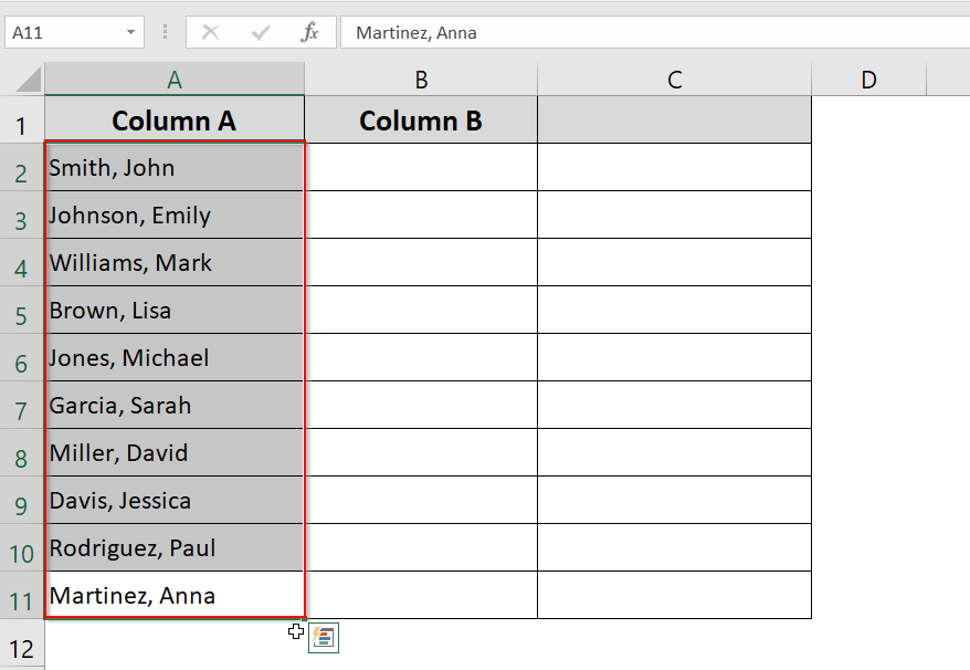
➤ Go to Data >> Text to Columns.
➤ Choose Delimited, then click Next.
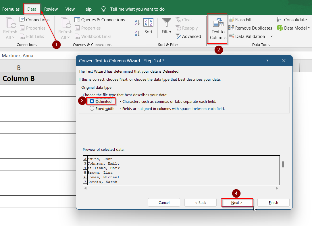
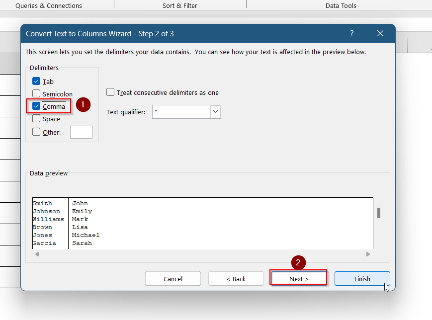
➤ Check the Comma delimiter and click Next.
➤ Click on Finish.
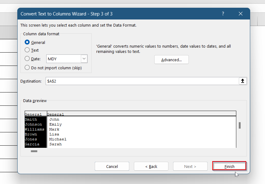
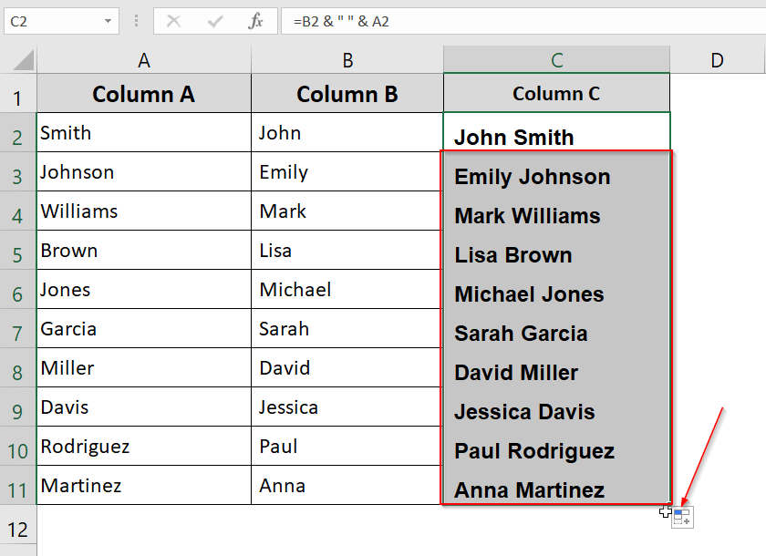
➤ Now the last and first names will be in separate columns (e.g., Column A and B).
➤ Add a new column (e.g., Column C) and enter this formula:
=B2 & ” ” & A2
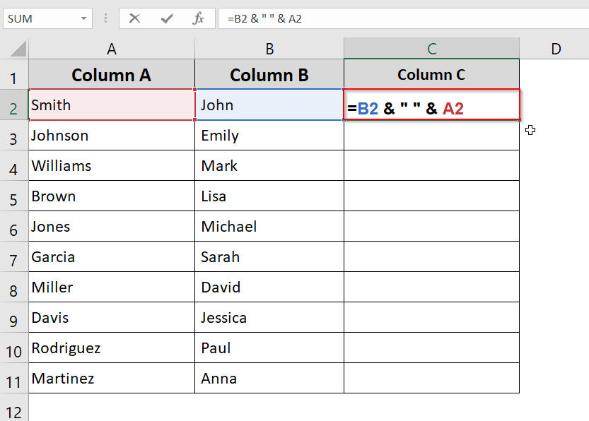
➤ Drag down to apply to the rest of the names.
Frequently Asked Questions
Can Excel reverse names automatically?
Not completely, but Excel can come very close. Features like Flash Fill and Power Query allow you to automate the process after giving an example or setting it up. You still need to guide it once before it finishes the rest.
What’s the fastest way to reverse names in Excel?
The fastest method is using Flash Fill. If your names follow a consistent format like “Last, First,” you just type the first reversed version manually, then press Ctrl + E to auto-complete the rest. It’s quick, accurate, and formula-free.
Can I reverse names without using formulas?
Yes, you can reverse names without writing any formulas. Excel tools like Flash Fill and Text to Columns offer visual, click-based methods. These are perfect for quick formatting tasks or one-time corrections when working with clean, consistent name lists.
What should I do if my name list has inconsistent formatting?
Inconsistent formatting can make reversing names tricky. First, try to clean the data by standardizing delimiters like commas or spaces. Then use Flash Fill or Text to Columns for easier and more accurate rearranging.
Wrapping Up
Reversing names in Excel may seem complex at first, but with the right tools and techniques, it’s easy to clean up and format your data. Whether you’re using formulas or Flash Fill, you can turn messy name columns into polished lists ready for printing, emailing, or exporting. Choose the method that fits your needs, and you’ll never have to manually retype a name again.