Conditional formatting is a powerful Excel feature that helps highlight cells based on specific conditions, making data easier to analyze at a glance. Sometimes, you want to format cells not just based on their own values but also depending on the contents of another cell. This becomes more interesting when you want to apply formatting based on multiple values in that other cell.
In this article, you’ll learn how to apply conditional formatting rules in Excel where formatting depends on multiple possible values in a different cell. Whether you’re working with text, numbers, or dates, these step-by-step methods will help you dynamically highlight cells and keep your spreadsheets clear and insightful.
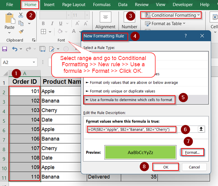
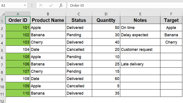
Steps to apply Conditional Formatting based on another cell with multiple values:
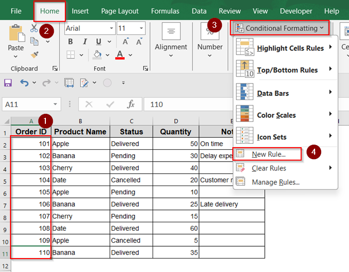
➤ Select the range you want to format (e.g., A2:A11).
➤ Go to Home >> Conditional Formatting >> New Rule.
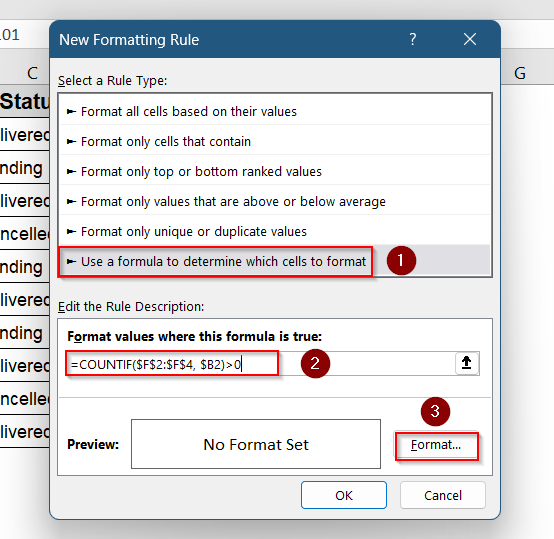
➤ Choose Use a formula to determine which cells to format.
➤ Enter the formula: =OR($B2=”Apple”, $B2=”Banana”, $B2=”Cherry”)
➤ From Format, pick your Fill color and click OK.
Using OR Formula for Multiple Text Values
If you want to highlight cells based on several possible values in another cell, the OR function inside a formula rule is perfect. For example, highlight cells in column A if the corresponding cell in column B contains “Apple“, “Banana“, or “Cherry“.
Steps:
➤ Select the range you want to format (e.g., A2:A11).
➤ Go to Home >> Conditional Formatting >> New Rule.

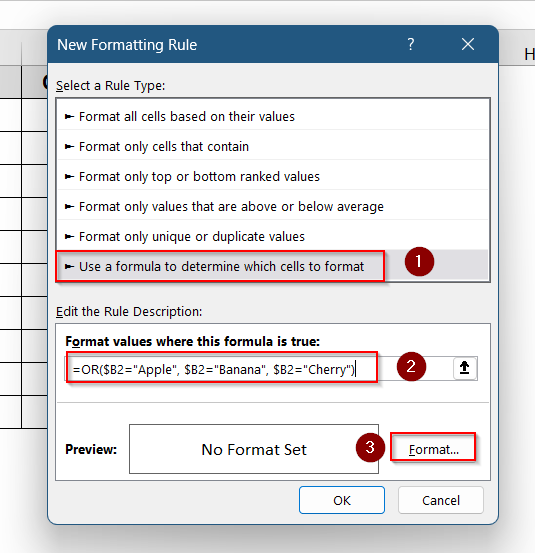
➤ Choose Use a formula to determine which cells to format.
➤ Enter the formula:
=OR($B2=”Apple”, $B2=”Banana”, $B2=”Cherry”)
➤ Click Format and pick your desired formatting style.
➤ Under fill, select your highlight color.(e.g., green).
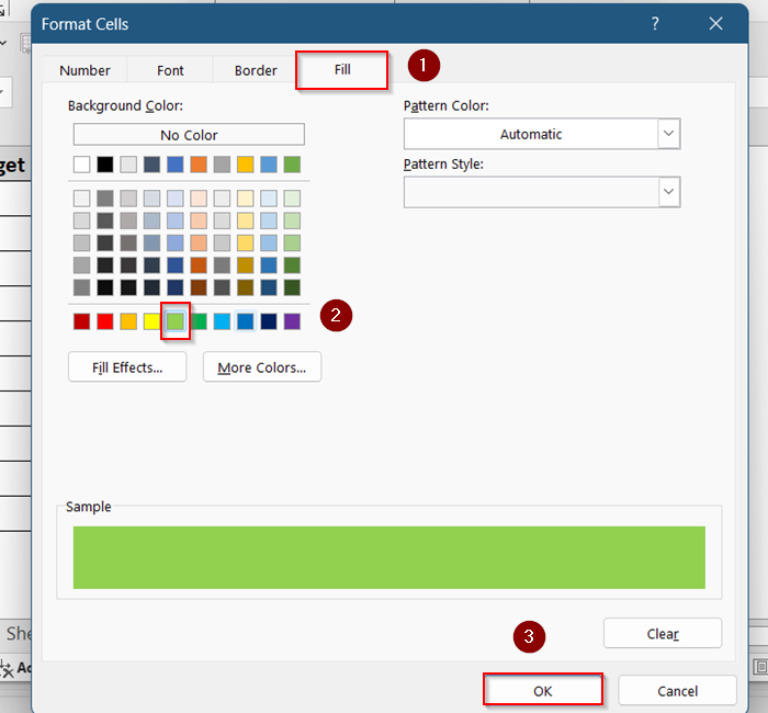
➤ Click OK to apply.
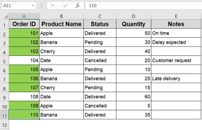
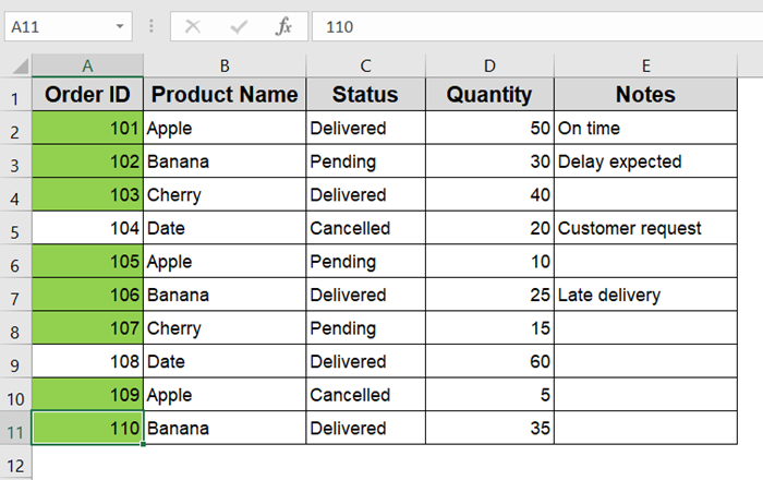
This rule checks each cell in column B and highlights the matching cells in column A accordingly.
Use COUNTIF for a List of Multiple Values
When you have many values to check, using COUNTIF with a list is more efficient than nesting many OR statements.
Steps:
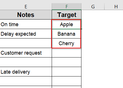
➤ First, create a list of values you want to check somewhere in your sheet, for example, in cells F2:F4.
➤ Select the range to format (e.g., A2:A11).
➤ Go to Conditional Formatting >> New Rule >> Use a formula to determine which cells to format.

➤ Enter this formula:
=COUNTIF($F$2:$F$4, $B2)>0
➤ Go to Format.
➤ Under fill, select your highlight color.(e.g., green).

➤ Click OK to apply.
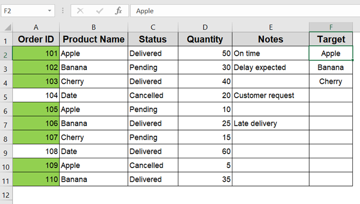
This formula highlights cells in column A when the adjacent cell in column B matches any value from your list.
Highlight Cells Based on Partial Matches (Contains Text)
Sometimes, the values in the other cell may contain text fragments rather than exact matches. Use the SEARCH or ISNUMBER function for this.
Steps:
➤ Select your target range (e.g., A2:A11).
➤ Go to Home >> Conditional Formatting >> New Rule.
➤ Choose Use a formula to determine which cells to format.
➤ Use the formula:
➤ Choose a format and press OK.
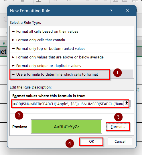
This highlights cells in column A when the adjacent cell in column B contains any of the specified substrings.
Using Named Range for Dynamic List of Values
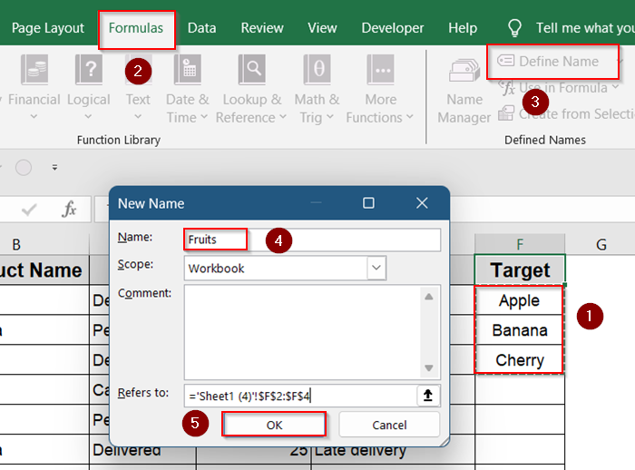
For better management of your list, create a named range.
Steps:
➤ Highlight your list cells (e.g., F2:F4), then go to the Formulas tab and click Define Name. Name it “Fruits“.
➤ Select your target range (e.g., A2:A11).
➤ Go to Home >> Conditional Formatting >> New Rule.

➤ Choose Use a formula to determine which cells to format.
➤ Use formula:
=COUNTIF(Fruits, $B2)>0
➤ Set formatting and confirm.
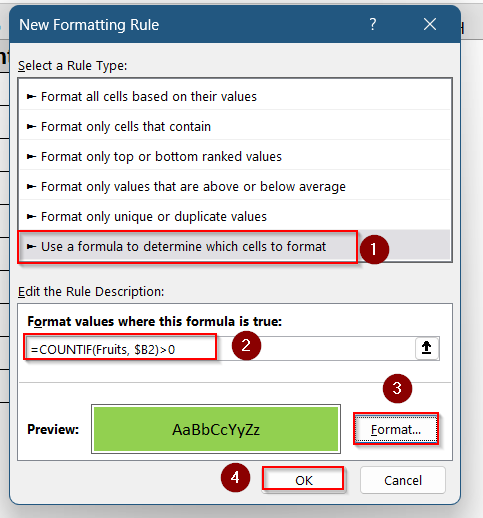
This makes your conditional formatting rule easier to maintain because you can just update the named range values when needed.
Frequently Asked Questions
Can I apply conditional formatting based on multiple values across different cells?
Yes. You can use complex formulas combining AND, OR, and COUNTIF to check multiple cells for various values, then apply formatting accordingly.
Does conditional formatting slow down Excel when using multiple formulas?
Large datasets with many conditional formatting rules can slow Excel’s performance. To optimize, limit ranges and prefer simpler formulas like COUNTIF over many nested OR statements.
Can I use conditional formatting to highlight based on numeric ranges in another cell?
Yes. For example, use a formula like =$B2>50 to highlight based on numeric values in adjacent cells.
What happens if I move or delete the list range used in COUNTIF?
If your list range changes, update the range reference or named range accordingly. Otherwise, formatting may stop working or highlight incorrect cells.
Is it possible to highlight cells if the other cell is blank or contains errors?
Yes, use formulas like =ISBLANK($B2) or =ISERROR($B2) inside conditional formatting rules to highlight those cases.
Wrapping Up
In this tutorial, we learned several ways to apply conditional formatting based on another cell’s value including exact text matches using OR, partial matches with SEARCH, and list-based checks with COUNTIF. These methods let you highlight relevant data quickly and keep your spreadsheet visually organized.
Feel free to download the sample file and experiment with each approach to see what works best for your data.