
In Excel, our dataset typically contains multiple categories, and we need to compare them to extract relevant information. In such a situation, using a pie chart is very useful as it allows us to visualize how different parts relate to the whole data. Also, this chart not only helps with interpreting the relationship, but it also helps us to determine the importance of each part.
Suppose you are analyzing sales for three different products across various regions. Now, to show how each product performs across regions, we can use a pie chart. Because a pie chart helps us to understand the sales contribution of each product in relation to the whole. So, we can easily visualize their relative shares and identify which products dominate in specific regions.
In this article, we will learn different methods to make a pie chart in Excel with multiple data sets, including the Recommended Charts tool, creating a Pivot Chart, and also making a Pie of Pie chart.
➤ First, select both of the columns of the dataset, i.e., A1 to B7 for our dataset.
➤ Then, click on the Insert tab from the upper menu bar and click on Recommended Charts from the Charts group.
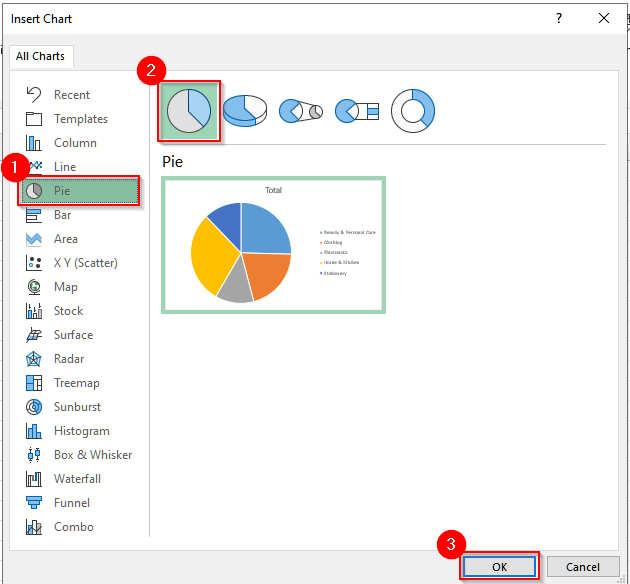
➤ Now, you will see a dialog box appear with different chart suggestions. Scroll to the Pie Chart option, choose it, and click OK.
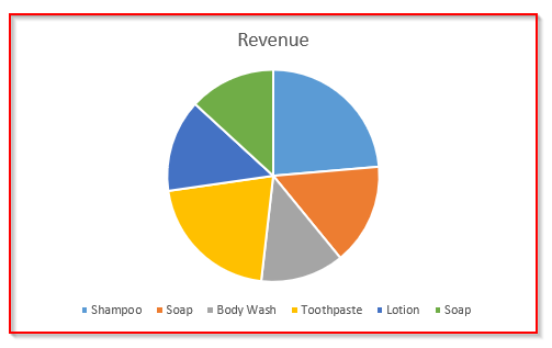
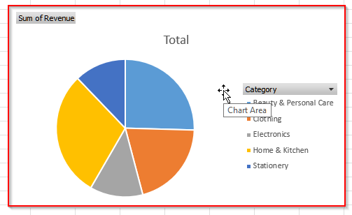
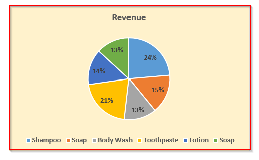
➤ Finally, you will see the pie chart.

Make a Pie Chart in Excel Using the Recommended Charts Tool
The Recommended Charts tool in Excel suggests a list of suitable charts for our data and helps us to quickly visualize the relationship among different categories.
We will use the dataset below to explain how you can make a pie chart with the Recommended Charts tool in Excel.
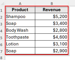
This is a simple dataset containing two columns, one for products and the other for their generated revenue.
Steps:
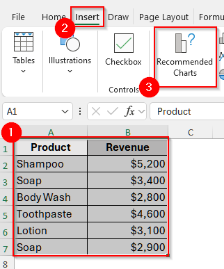
➤ First, select both of the columns of the dataset, i.e., A1 to B7 for our dataset.
➤ Then, click on the Insert tab from the upper menu bar and click on Recommended Charts from the Charts group.
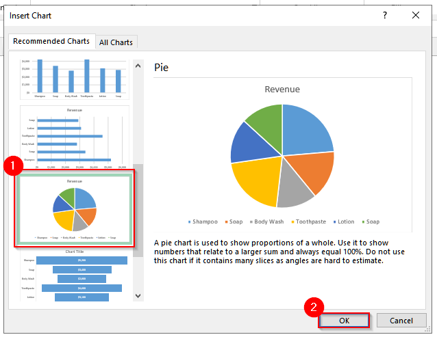
➤ Now, you will see a dialog box appear with different chart suggestions. Scroll to the Pie Chart option, choose it, and click OK.
➤ Finally, you will see the pie chart.
Create a Pivot Pie Chart with Multiple Data in Excel from Pivot Table
Using a Pivot Table, we can quickly group and summarize multiple sets of data without any formulas. Then we can turn that Pivot Table into a Pie Chart easily.
We will use the data below to explain how you can make a Pivot Table and then convert it into a Pie Chart in Excel with multiple data.
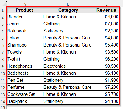
This is a department store dataset with a few products, their categories, and the revenue generated from them in a few days.
Steps:
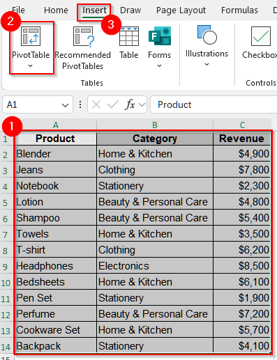
➤ First, select the whole dataset, i.e., A1 to C14, for our dataset.
➤ Then, go to the Insert tab from the upper menu ribbon and click on PivotTable.
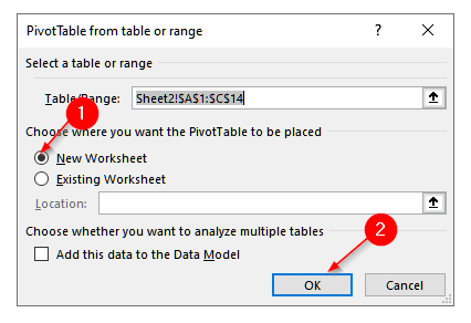
➤ Now, you will see a new dialog box. Choose New Worksheet from that pop-up and click OK.
➤ Then, drag Category into the Rows area from the PivotTable Fields pane.
➤ Also, drag Revenue into the Values area, and it will show the sum of the revenue per category.
➤ Now, click anywhere inside the Pivot Table and go to Insert and then select PivotChart.
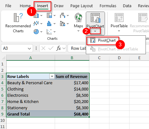
➤ A new window will open up with a list of chart options. Select Pie Chart from that list and click OK
➤ Now, you will see the Pie Chart.
Make a Pie of a Pie Chart with Multiple Data in Excel
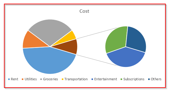
When our data has too many small divisions or categories, the slices of our pie chart become dense and smaller. And it becomes hard for us to see the smaller divisions clearly. Also, when our dataset includes the cost or revenue of main divisions and their corresponding smaller categories, we cannot display those smaller categories alongside the divisions and their associated costs. In such cases, a pie of a pie chart helps us create a small pie chart with fine divisions and improve the visualization.
We will use the dataset below to show how you can make a pie of a pie chart to show the smaller categories clearly.
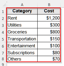
In our dataset, we have 7 categories of household breakdown, among which a few are very low.
Steps:
➤ First, select the whole dataset, i.e., cell A1 to C9 for our dataset.
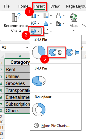
➤ Then, go to Insert and from the Charts division, select the icon for a Pie or Donut chart, and then select the 2nd pie chart option under the 2-D Pie.
➤ Now, you will see the pie of a pie chart where one the second pie chart, the categories with low values are shown clearly.
Formatting the Pie Chart
Now, to make our pie chart clearer and more presentable, we will format the first chart by adding data labels, percentages, and editing the color.
Add Data Labels And Percentages
Data labels help us to identify a category easily and quickly. So, we will add the data labels of our pie chart now.
Steps:
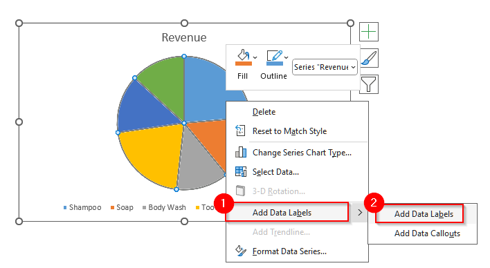
➤ First, right-click on the pie chart, and you will see a box pop out with a few options.
➤ Select Add Data Labels and then click on Add Labels.
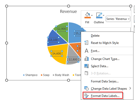
➤ Now, you will see the default values as the data labels. To make the contribution of the categories to the whole clearer, we will change the values to show the percentages now. Right-click on any data label and select Format Data Labels.
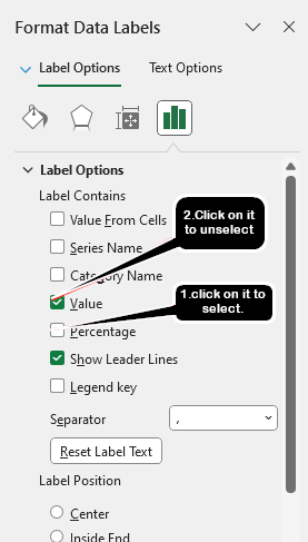
➤ You will see a new window open up at the rightmost side of your dataset. In it, first click on the Percentages to select it, and then click on the Values to deselect it.
Edit the Color of the Pie Chart
Now, we will edit the color of our pie chart to make it visually more appealing.
Steps:
➤ First, click on any area on the chart, and you will see a new option called Chart Design on the upper menu bar.
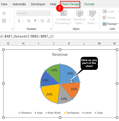
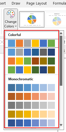
➤ Now, click on the Chart Design and select the Change Color option to choose a preset color set.
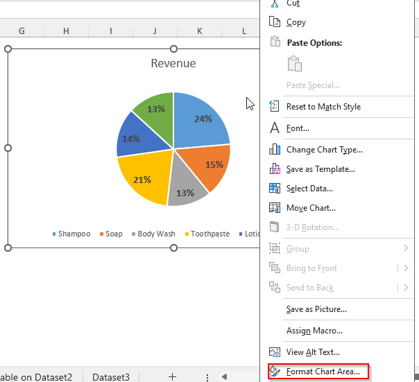
➤ You can also change the background color of the chart. To do it, right-click on the chart area, and it will open up a list of options.
➤ Now, select Format Chart Area, and a new tab will open up.
➤ Then, choose the fill type from the Fill option and choose a color from the Color option.
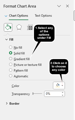
➤ Finally, the pie chart’s customization is complete.
Frequently Asked Questions
Can I Make a Pie Chart With Three Variables in Excel?
It depends on the type of variables. If you have two categorical variables among the three variables, you can create a pie chart with all the variables. However, if you have more than one numerical variable, you cannot. Because, a pie chart can only represent one set of numerical values at a time, and each slice shows its proportion of the total. So, you cannot have more than one set of numerical variables in a single pie chart.
Wrapping up
In this article, we have learned to make a pie chart in Excel with the built-in Recommended Charts option and with the PivotTable. We have also learned how to make a pie of a pie chart and format a pie chart. Try these methods and reach out to us if you have any inquiries.