
Managing business performance requires comparing budgeted and actual results. This article explains budget vs actual variance and teaches how to calculate the budget vs. actual variance formula in Excel. In addition, to visualize the results, we’ll plot a budget vs actual variance chart in Excel and learn to highlight budget vs actual variances with Conditional Formatting. Whether you’re tracking project costs, revenue, or expenses, this approach will help you analyze and communicate financial results.
➤ Budget vs actual variance is the difference between the planned and the actual amount. In this article, we’ll learn about budget vs actual variance, how to calculate the budget vs actual variance formula in Excel, and plot a budget vs actual variance chart in Excel.
➤ Variance formula: =Actual value-Budgeted value
➤ Variance % formula: =(Actual value-Budgeted value)*100/Budgeted value
➤ Variance % chart: Select data >> Insert >> Column or Bar Chart >> Clustered Column.
➤ Conditional Formatting Variance %: Select data >> Conditional Formatting >> New Rules >> Use formula to determine which cells to format >> Enter formula >> Format >> Fill >> Color >> OK.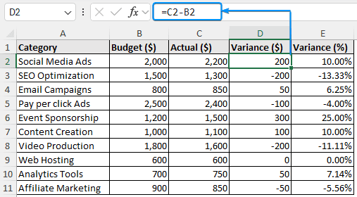
What is Budget vs Actual Variance?
Budget vs. actual variance is the difference between the planned (budgeted) and what was actually spent. It is a fundamental financial analysis instrument that helps monitor performance and identify over spending or under spending.
➤ Positive variance: You made more money or spent less than you planned. Positive variance is favorable.
➤ Negative variance: You made less money or spent more than you had planned. Negative variance is unfavorable.
Budget vs Actual Variance Formula
There is a simple formula to measure the difference between the planned and actual value i.e. budget vs actual variance.
Variance: =Budgeted amount-Actual amount
Budget vs Actual Variance Percentage Formula
The budget vs actual variance value can be expressed as a percentage. Some of the key benefits of expressing the variance as a percentage are:
➤ Percentage normalizes the value, making comparisons easier.
➤ Large percentages are easy to identify and understand.
Variance %: =(Budgeted amount-Actual amount)*100/Budgeted amount
Calculating Budget vs Actual Variance in Excel
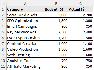
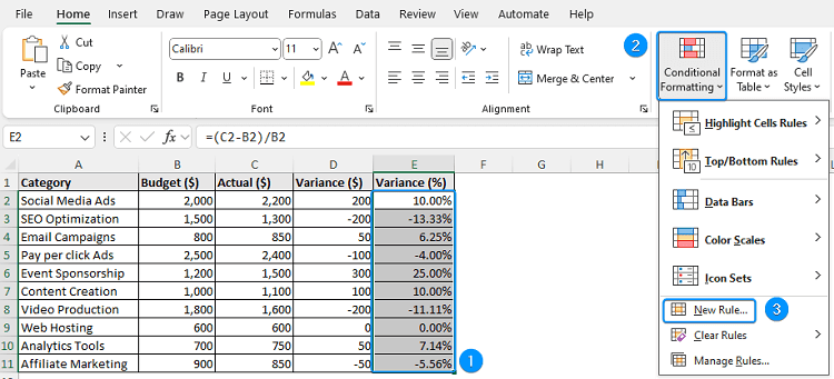
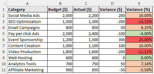
The marketing and operational expense dataset contains the category, budget amount in dollars, and the actual amount spent in dollars from columns A through C.
Consider creating a report to assess which marketing strategies were successful in staying within budget and which ones went over budget. To easily identify the trouble spots, we calculated both variance and percentage variance.
For example, you are considering the Event Sponsorship budget. The actual cost was $1,600, even though you had originally budgeted $1,300. A 23% over budget for event sponsorship indicates a considerable unfavorable deviation. To maintain a threshold of ±5%, further research is needed. It is possible that costs were understated or that unforeseen fees were incurred. Now, let’s apply the arithmetic formula in Excel to calculate the variance and percentage variance.
Steps:
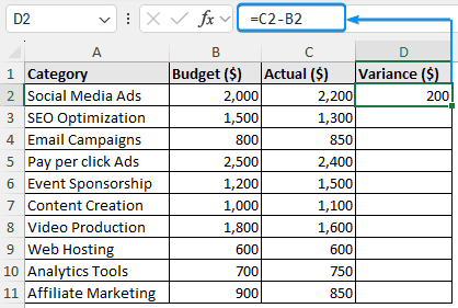
➤ Select the output cell (D2) and enter the budget vs actual variance formula.
=C2-B2
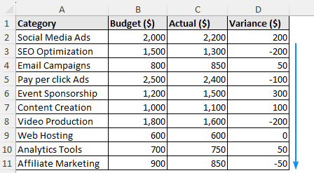
➤ Use the Fill Handle tool to copy the formula to the cells below.
➤ To calculate the percentage variance, use the budget vs actual variance percentage formula. Apply percentage formatting to the cells.
=(C2-B2)/B2
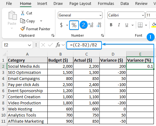
➤ Auto fill the formula to the rest of the cells.
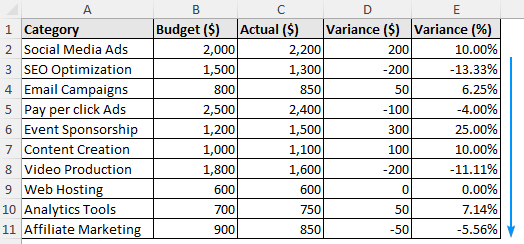
➤ SEO optimization and video production were both under budget and saved the most money.
➤ Web hosting showed no difference. The budget and actual spending were the same.
It is easier to modify strategies and keep expenses under control when variances are visualized. In the next we’ll learn to plot the budget vs actual variance chart.
Budget vs Actual Variance Chart
A budget vs actual variance chart quickly identifies the differences by comparing each category’s budgeted and actual amounts. This chart simplifies the determination of the categories that are over budget or under budget. This approach is ideal for presentations, reports, or monthly reviews and is particularly useful to stakeholders who prefer data visualization over spreadsheets. Let’s use a clustered column chart to visualize the data. This chart is located in the Insert tab under the column or bar chart group.
Steps:
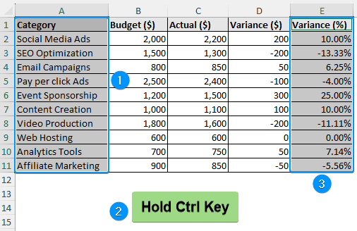
➤ To plot the budget vs actual variance chart, highlight the category and variance % columns from the two non-contiguous/non-adjacent cell ranges.
➤ Select the first cell range (A1:A11), hold down the Ctrl key and choose (E1:E11) range.
➤ Go to the Insert tab >> Column or Bar Chart >> Clustered Column.

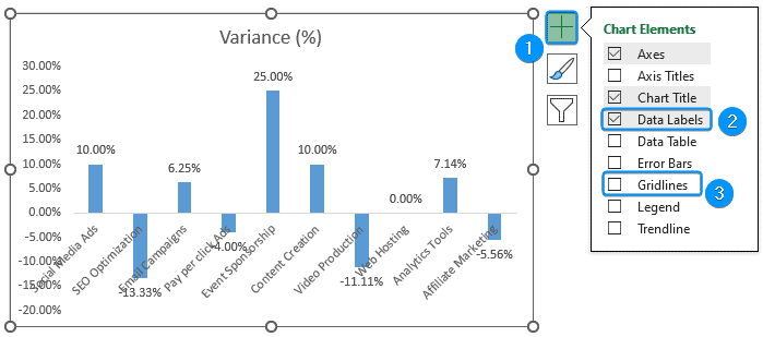
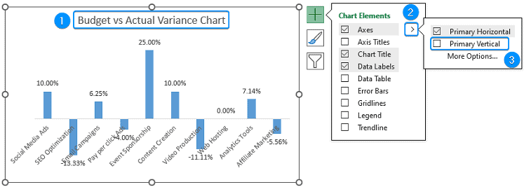
➤ Click Chart Elements (plus icon) >> Uncheck Gridlines >> Check Data Labels.
➤ Provide a suitable chart title >> Click the arrow beside Axis option >> Deselect Primary Vertical axis.
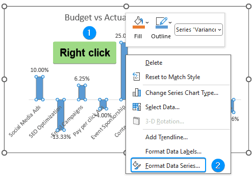
➤ Right click on any of the columns >> Format Data Series.
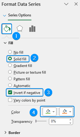
➤ In the Format Data Series pane, Fill & Line (paint bucket icon) >> Expand the Fill section >> Solid fill >> Invert if negative >> Select suitable colors.
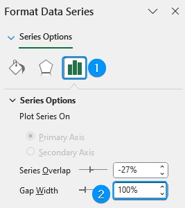
➤ Click Series Options >> Set the Gap width to 100%.
➤ The chart is ready.
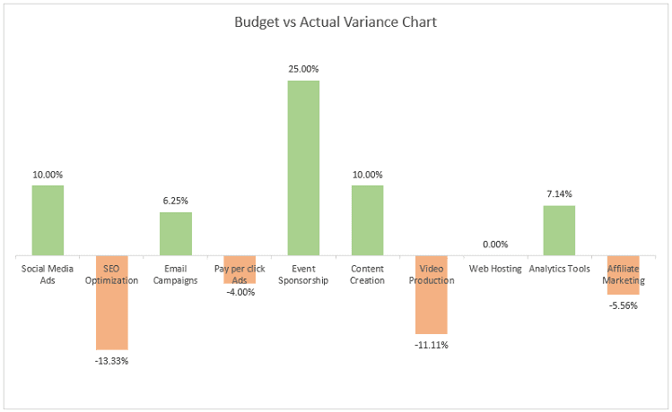
The results have been discussed previously.
Highlight Variance Percentage with Conditional Formatting
Excel’s Conditional Formatting feature lets you color code the % variance column for a quick visualization of the budget variance. Without any calculations or filters, you can spot which budget items are within the acceptable range and which need action.
Steps:
➤ Select the range (E2:E11) >> Conditional Formatting >> New Rules.
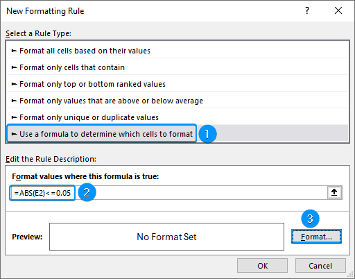
➤ Use a formula to determine which cells to format >> Enter the formula for highlighting variances less than 5% >> Format.
=ABS(E2)<=0.05
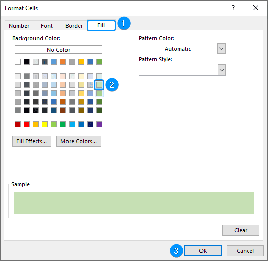
➤ Fill section >> Choose a fill color (Green) >> OK.
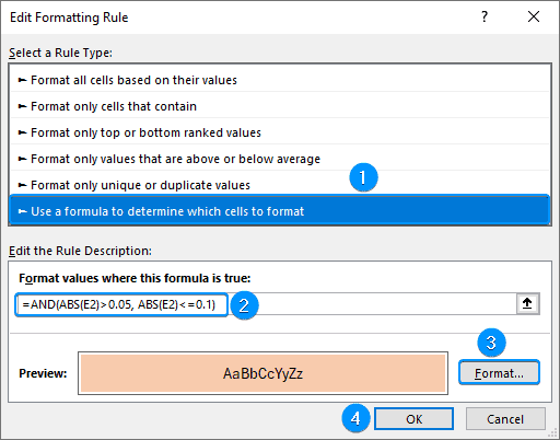
➤ Use a formula to determine which cells to format >> Type the formula to highlight variances between 5 and 10% >> Format (select orange fill color).
=AND(ABS(E2)>0.05, ABS(E2)<=0.1)
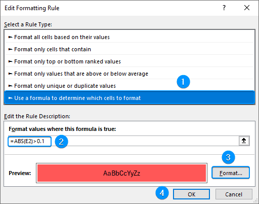
➤ Use a formula to determine which cells to format >> Enter the formula to highlight variances that exceed 10% >> Format (select red fill color).
=ABS(E2)>0.1
➤ The variances have been formatted based on the set conditions.
➤ Moderate overspend or underspend is indicated by orange (±5% to ±10%), indicating manageable problems.
➤ Critical variations (over ±10%) are highlighted in red, warning of possible errors in budget planning, unforeseen or unaccounted expenses.
Frequently Asked Questions
How do I calculate budget vs. actual variance in Excel?
Variance: =Actual value-Budgeted value
How can I calculate the percentage variance?
Percentage Variance: =(Actual value-Budgeted value)*100/Budgeted value
What does a positive and negative variance indicate?
A positive variance indicates the actual amount is greater than the budgeted amount. Meanwhile, a negative variance represents that the actual amount is less than the budgeted amount.
What is the formula for actual cost variance?
Actual cost variance: =Actual cost-Budgeted cost
What is the acceptable range for variance?
Typically, a variance of ±5% is acceptable. However, it varies based on the industry and the type of cost.
Wrapping Up
In this tutorial, we’ve learned about budget vs actual variance, budget vs actual variance formula in Excel. Moreover, we calculated the percentage variance, budget vs actual variance chart, and explored highlighting percentage variance with Conditional Formatting. Feel free to download the practice file and share your thoughts and suggestions.