When working with large Excel datasets, it’s often crucial not just to find the maximum value but also to identify exactly where it is located. Whether you’re tracking sales, scores, or other metrics, finding the max value and its cell address lets you quickly locate key data points for further analysis.
In this article, we’ll learn several effective methods to get the max value and the corresponding cell address using Excel functions like MAX, INDEX/MATCH, CELL, ADDRESS, XLOOKUP, TEXTJOIN and VBA for advanced cases. Each method includes clear step-by-step instructions suiting various needs and different Excel versions.
Steps to find the max value and corresponding cell in Excel:
➤ Select a blank cell like G3.
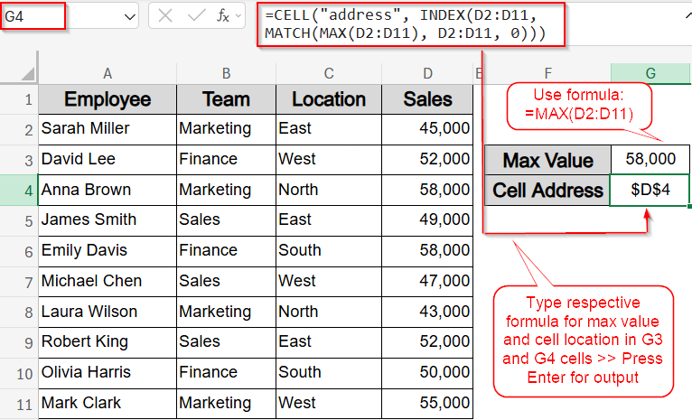
➤ Enter this formula:
=MAX(D2:D11)
➤ Press Enter to get the max value (58,000).
➤ In another cell like G4, enter this formula to get the cell address:
=CELL(“address”, INDEX(D2:D11, MATCH(MAX(D2:D11), D2:D11, 0)))
➤ Press Enter to display output like $D$4.
Find Max Value and Cell Address Using INDEX, MATCH and CELL Functions
This method combines INDEX, MATCH, and CELL functions to find the maximum value and the exact cell address where it appears. Once applied, the formulas will display both the highest value such as 58,000 and its cell address like $D$4 which will give you a complete picture in a few steps.
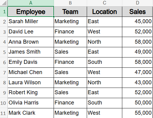
To demonstrate the formulas clearly, we’ll use a sample dataset containing employee information with columns for Employee Name, Team, Location, and Monthly Sales. This setup lets us find the highest sales figure and the corresponding cell location efficiently.
Steps:
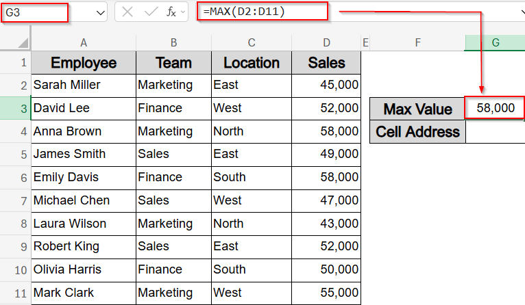
➤ Select a blank cell like G3.
➤ Enter this formula:
=MAX(D2:D11)
➤ Press Enter to get the max value (58,000).
➤ In another cell like G4, enter this formula to get the cell address:
=CELL(“address”, INDEX(D2:D11, MATCH(MAX(D2:D11), D2:D11, 0)))
➤ Press Enter.
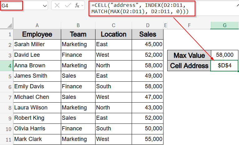
Now you’ll see the cell address $D$4 which is the cell location of the first max value.
Get Max Value and Cell Address Using Aggregate and ADDRESS Functions
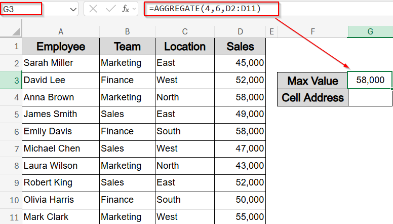
This method uses the AGGREGATE function to find the maximum value and the ADDRESS function to return the exact cell where it’s located. It’s a great option for skipping hidden rows and dynamically identifying the top value like 58,000 and its cell address, such as D4.
Steps:
➤ In a blank cell like G3, type thai formula to get the max value:
=AGGREGATE(4,6,D2:D11)
➤ Press Enter.
➤ Select a blank cell like G4.
➤ Type this formula:
=ADDRESS(MATCH(MAX(D2:D11), D2:D11, 0) + ROW(D1), COLUMN(D1), 4)
➤ Press Enter.
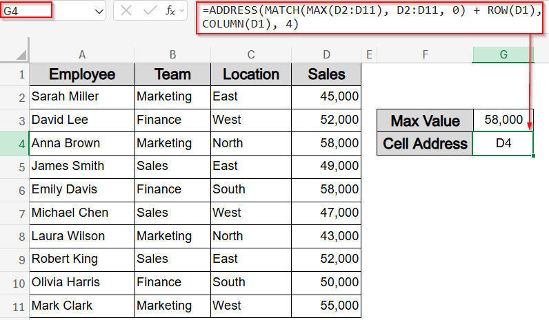
The formula returns D4 which is the exact cell of the first maximum sales.
Return Max Value and Cell Address Using LARGE, XLOOKUP and CELL Functions (Excel 365)
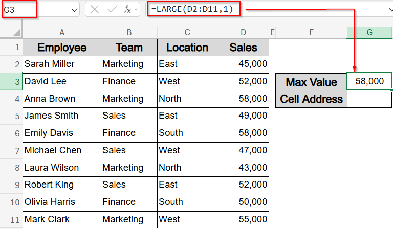
If you’re using Excel 365, this modern method combines the LARGE, XLOOKUP, and CELL functions to retrieve the highest salary and its exact cell address from your dataset. It’s ideal for quickly pinpointing not just the top value but where it resides in the sheet. In our sample dataset range D2:D11 representing Monthly Sales, this technique helps identify the top salary and shows its position clearly.
Steps:
➤ Select a blank cell like G3.
➤ Enter this formula for the max value:
=LARGE(D2:D11,1)
➤ Press Enter for output (58,000).
➤ In the next cell (G4), get the cell address of the max value using this formula:
=CELL(“address”, XLOOKUP(MAX(D2:D11), D2:D11, D2:D11))
➤ Press Enter.
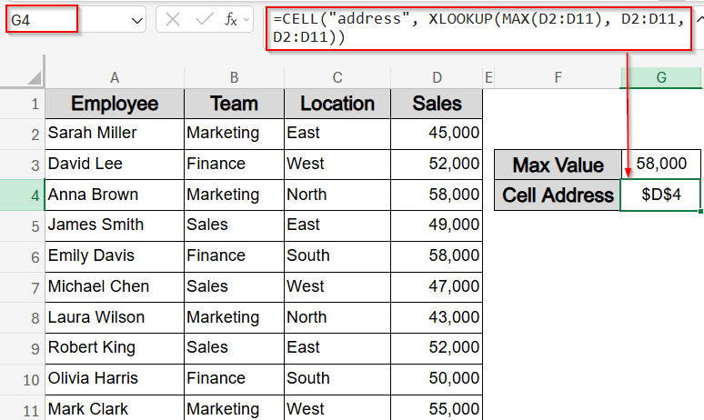
Now the cell address $D$4 appears pulled directly from column D where the max sales are located.
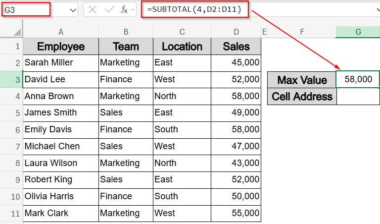
Use SUBTOTAL, LET and XLOOKUP Functions for Max Value and Cell Address
This method is perfect for advanced users who want a cleaner, more efficient way to retrieve the maximum value and its cell address using Excel 365’s dynamic formula features. The SUBTOTAL function gets the max value while LET function defines reusable variables, and XLOOKUP function locates the value’s position. Let’s proceed to find the maximum Sales value and it’s cell position using formulas.
Steps:
➤ In a blank cell like G3, type this formula to get the max value:
=SUBTOTAL(4,D2:D11)
➤ Press Enter.
➤ Select a blank cell like G4.
➤ Enter this formula:
=LET(range, D2:D11, maxVal, MAX(range), cellRef, XLOOKUP(maxVal, range, range), ADDRESS(ROW(cellRef), COLUMN(cellRef), 4))
➤ Press Enter.
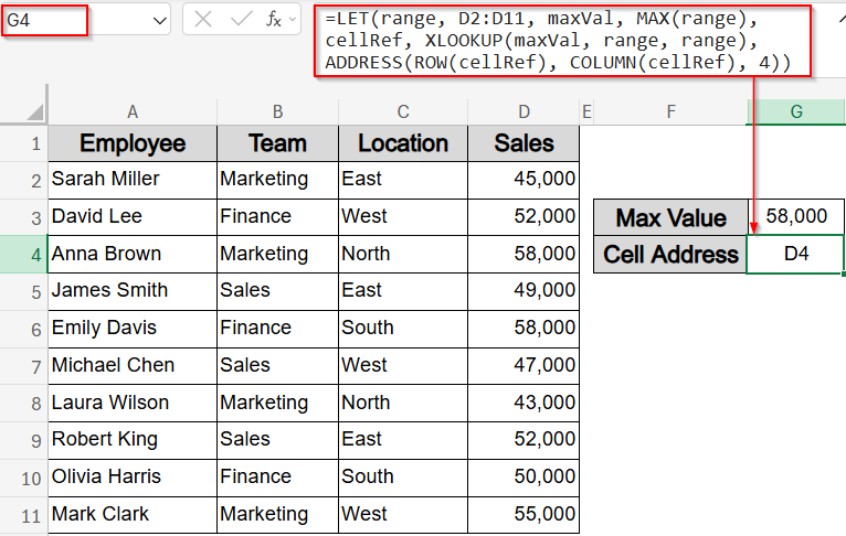
This formula returns D4 cell which is the max value’s cell location.
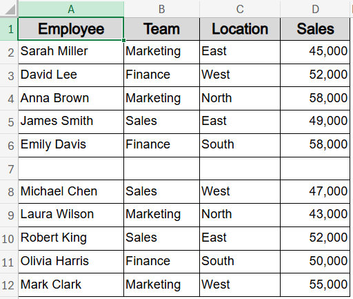
Find Max Value and Cell Address Across Non-Adjacent Ranges
When working with fragmented datasets, the maximum value may lie across non-adjacent blocks of rows. In such cases, you can combine the MAX, INDEX, MATCH, and CELL functions to accurately detect the highest value and its exact position. This method is ideal when rows are hidden or filtered out or your table is split by design.
Based on the dataset below, the formulas identify the first max salary which is 58,000 and returns the corresponding cell address $D$4.
Steps:
➤ Select a blank cell like G3.
➤ Enter this formula to find max value in two ranges:
=MAX(D2:D6, D8:D12)
➤ Press Enter (returns 58,000).
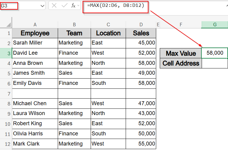
➤ To get the cell address of the max value in the full range, use this formula in G4 cell:
=CELL(“address”, INDEX(D2:D12, MATCH(MAX(D2:D6, D8:D12), D2:D12, 0)))
➤ Press Enter.
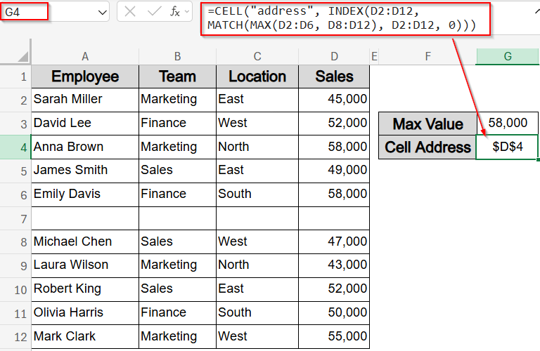
Now the maximum value along with it’s cell location is visible to you.
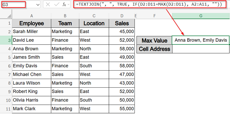
Find Multiple Max Value Entries and Cell Locations with TEXTJOIN Function
If multiple entries share the highest value, this method lists all corresponding names in a single cell separated by commas. The output consolidates all top performers, providing a quick overview of ties. For example, we will get two top employees with the same amount of maximum Sales and their cell addresses by applying formulas.
Steps:
➤ Select a blank cell like G3.
➤ Enter this formula to list all employees tied for the max salary:
=TEXTJOIN(“, “, TRUE, IF(D2:D11=MAX(D2:D11), A2:A11, “”))
➤ Press Ctrl + Shift + Enter in older Excel, or just Enter in Excel 365.
➤ To get the cell references of max salaries, use this formula in G4 cell:
=TEXTJOIN(“, “, TRUE, IF(D2:D11=MAX(D2:D11), “D” & ROW(D2:D11), “”))
➤ Press Ctrl + Shift + Enter in legacy Excel, or just Enter in modern versions.
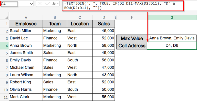
Now all employees sharing the maximum sales are listed with their corresponding cell locations.
Find Max Value with Single or Multiple Conditions
When working with filtered data, you might want to find the highest value based on one or more conditions like identifying the top salary in the Sales department, or the highest amount from a specific region and team. This method uses the IF function with MAX to apply logic-based filtering and return the correct maximum. It’s useful for conditional analysis when your dataset includes categories like Department and Region.
In this example, we will find the maximum value for the Sales team showing both single and multiple criteria.
Steps:
➤ Select a blank cell like G4.
➤ Enter this array formula to find the max salary for Sales department:
=MAX(IF(B2:B11=”Sales”, D2:D11))
➤ Press Ctrl + Shift + Enter in older Excel and just Enter in Excel 365.
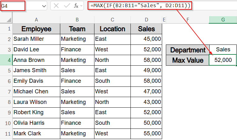
➤ For multiple conditions, use this formula to find max value from Sales department in the East region:
=MAX(IF((B2:B11=”Sales”)*(C2:C11=”East”), D2:D11))
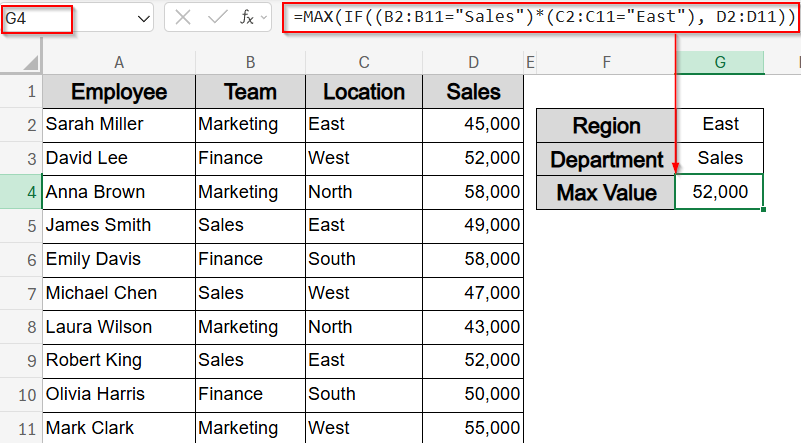
Now you have filtered your data based on multiple criteria to derive the maximum sales value which is 52,000.
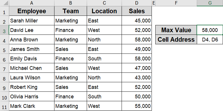
Apply VBA Macro to Find Max Value and All Corresponding Cell Addresses
If you’re working with large or irregular datasets where the maximum value may appear more than once, a VBA macro can automatically identify and list all cells that contain that maximum. This is especially helpful for audits or summaries that require precise locations of high values.
In this case, the output returns the maximum value and their cell addresses like D4 and D6 separated by a comma.
Steps:
➤ Press Alt + F11 to open the VBA editor.
➤ Insert a new module using Insert tab >> Module.
➤ Paste the following code:
Sub Find_Max_Value_and_Cell_Addresses()
    Dim rng As Range
    Dim maxVal As Double
    Dim addresses As String
    Dim cell As Range
    Dim outputCell As Range
    Set rng = Application.InputBox("Select range:", Type:=8)
    maxVal = Application.WorksheetFunction.Max(rng)
    For Each cell In rng
        If cell.Value = maxVal Then
            addresses = addresses & cell.Address(False, False) & ", "
        End If
    Next cell
    If Len(addresses) > 0 Then
        addresses = Left(addresses, Len(addresses) - 2) ' Remove trailing comma
    End If
    Set outputCell = Application.InputBox("Select output cell:", Type:=8)
    outputCell.Value = maxVal
    outputCell.Offset(1, 0).Value = addresses
End Sub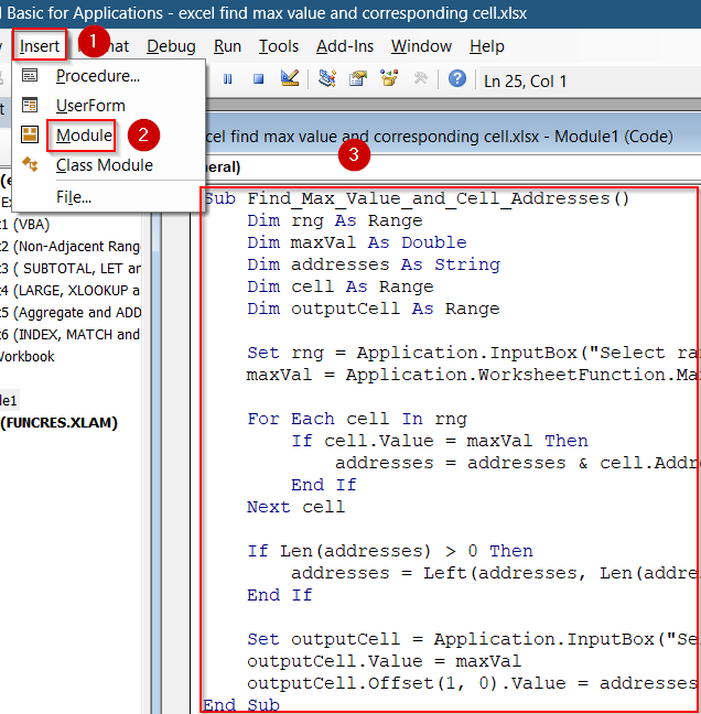
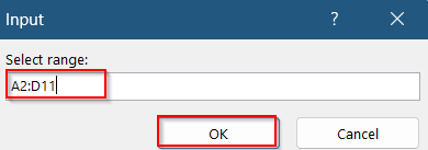
➤ Run this macro by pressing F5 key. Select your range from the pop-up dialog and click OK.
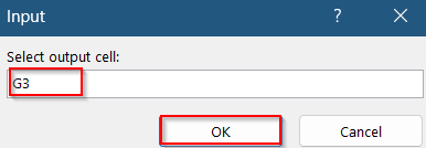
➤ You will be prompted again to confirm your output cell such as G3 and hit OK.
Now you’ll find your max value and all corresponding cell addresses in the selected location. Optionally, format your results according to your choice.
Frequently Asked Questions
Does the TEXTJOIN function require Ctrl + Shift + Enter ?
In Excel 365 and Excel 2021, TEXTJOIN function works as a dynamic array function and needs only Enter. However, in older Excel versions, it must be entered as an array formula using Ctrl + Shift + Enter .
Can I apply multiple conditions when finding the max value?
Yes, use MAX and IF functions with multiple logical tests. Combine conditions using multiplication (*) for AND logic or addition (+) for OR logic to filter the range before calculating the max value.
Why should I use SUBTOTAL instead of MAX in some cases?
SUBTOTAL function ignores filtered or manually hidden rows, unlike MAX. This is useful when working with filtered reports or dashboards where you want to calculate max based only on visible values, keeping results dynamically updated.
What’s the advantage of using LET with XLOOKUP?
The LET function defines reusable names for parts of your formula, improving readability and performance. When used with XLOOKUP function, it simplifies complex logic and allows for cleaner extraction of the max value and its position in one step.
Wrapping Up
In this tutorial, we explored how to find the maximum value and its corresponding cell in Excel using various approaches from basic MAX functions to advanced formulas with LET, XLOOKUP, and even VBA. Each method helps you pinpoint not just the top value but also where it exists in your sheet. Whether you’re working with filtered data, multi-block ranges, or duplicate entries, you now have the tools to extract and highlight peak data points efficiently. Feel free to download the practice file and share your feedback.