When working with data in Excel, you often need to add values based on more than one condition. For example, you might want to total sales only when the Product is “T-Shirt” and the Region is “East”. These criteria come from different columns, so a basic SUMIF function won’t be enough.
The more convenient way is to use functions like SUMIFS and SUMPRODUCT, that allow you to apply multiple conditions across separate columns. These functions help you filter your data more precisely and calculate totals based on specific combinations.
You can apply these methods in Excel by setting up a formula that checks each column for a match, then sums the values that meet all conditions. In this article, we’ll show you how to do that step by step using a real dataset.
To sum sales with the SUMIF function, first we have to create a helper column that combines both conditions into one text string. Then we can apply the function with multiple criteria for different columns in Excel.
Here’s how to apply this method:
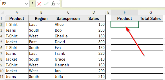
➤ Open your dataset in Excel.
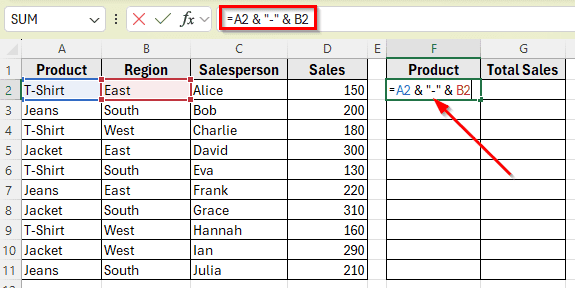
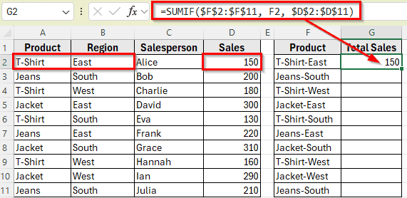
➤ To create helper column, insert a formula that combines Product and Region in cell F2:
=A2 & “-” & B2
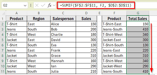
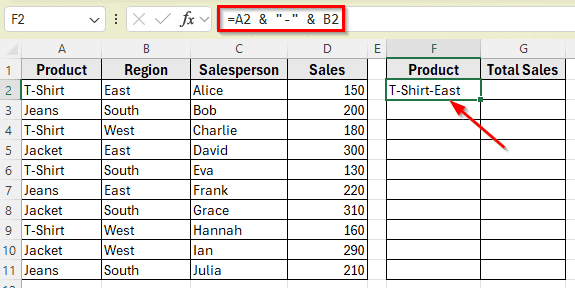
➤ Now the rows will look like T-Shirt-East, Jeans-South, etc.
➤ Now, type this formula in cell G2
=SUMIF($F$2:$F$11, F2, $D$2:$D$11)
➤ Press Enter. You’ll see the result of total sale in cell G2, which is 150.
➤ Drag the formula across the matrix to fill other cells.
Using SUMIFS Function to Sum with Multiple Criteria from Different Columns
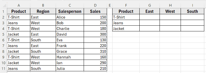
In the following dataset, we have a product sales list that includes item names, sales regions, salespersons, and total sales. There are four main columns: Product, Region, Salesperson, and Sales. Column A lists the product types, Column B shows the region where each sale occurred, Column C contains the salesperson’s name, and Column D records the sales amount.
We’ll use this dataset to calculate the total sales for each product and region combination listed in the summary table starting from Column F. The goal is to sum the values in Column D only when the product in Column A matches the row header and the region in Column B matches the column header. The results will appear in the empty cells of the matrix, allowing you to see total sales by both product and region.
The simplest and most reliable way to apply multiple conditions in Excel is by using the SUMIFS function. Unlike SUMIF, which handles only one condition, SUMIFS function allows you to check multiple columns at the same time.
In this method, we want to calculate the total sales for each combination of Product and Region using this formula. We’ll add up the values in the Sales column only when both the Product and Region match the headers in the summary table.
Here’s how to apply this method:
➤ Open your dataset in Excel.
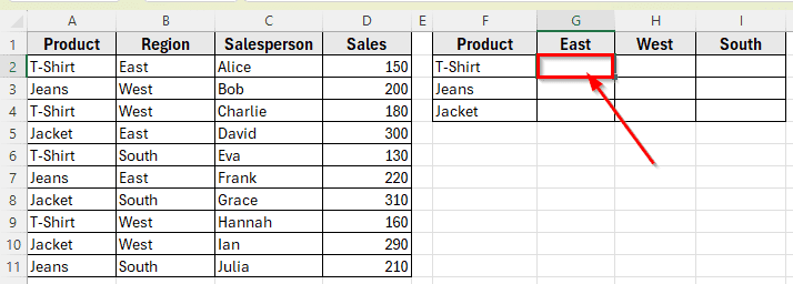
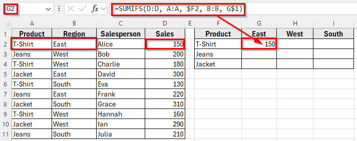
➤ Click on cell G2 in the summary table, where you want to calculate the total sale for T-Shirt in the East region.
➤ Type the following formula
=SUMIFS(D:D, A:A, $F2, B:B, G$1)
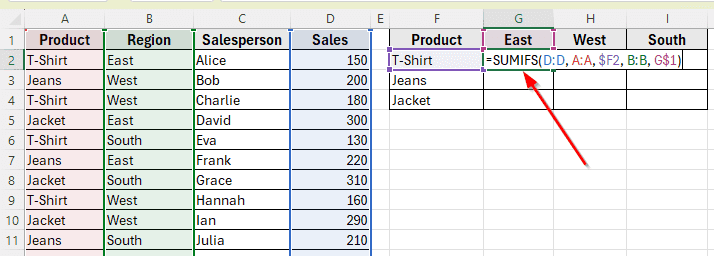
➤ Press Enter. This will return the total sales where Product is T-Shirt and Region is East.
The use of $F2 locks the column while copying the formula across columns, and G$1 locks the row while dragging it down. This way, each formula references the correct Product and Region from the summary table.
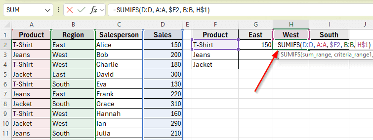
➤ Now for the other two regions such as West and South, you have to enter a similar formula. For example, for the West region, enter this formula in cell H2:
=SUMIFS(D:D, A:A, $F2, B:B, H$1)
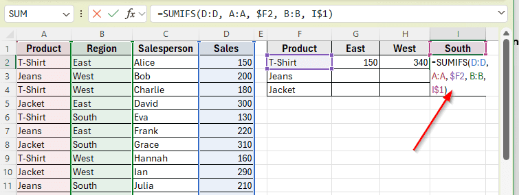
➤ Next, for the South region, enter this formula in cell I2:
=SUMIFS(D:D, A:A, $F2, B:B, I$1)
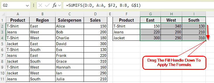
➤ After entering the formula in G2, H2, I2, drag it across and down the summary table to fill the rest of the cells.
➤ Each result will update automatically based on the matching Product and Region.
Applying SUMIFS Function in a Matrix Layout
Another convenient way to apply multiple criteria across different columns is by using the SUMIFS function in a matrix-style layout. This method allows you to create a summary table where the rows represent one condition such as Product, and the columns represent another such as Region. Each cell in the table shows the total sales for that specific combination.
Here’s how to apply this method:
➤ Open your dataset in Excel.
➤ Make sure you have Products listed vertically in Column F and Regions listed horizontally in Row 1 (starting from G1).
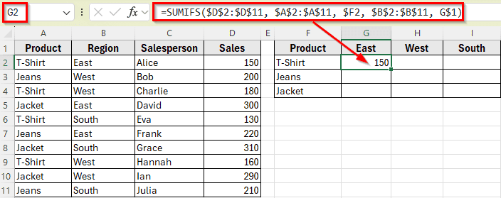
➤ Click on cell G2, where the row is T-Shirt and the column is East.
➤ Type the following formula
=SUMIFS($D$2:$D$11, $A$2:$A$11, $F2, $B$2:$B$11, G$1)
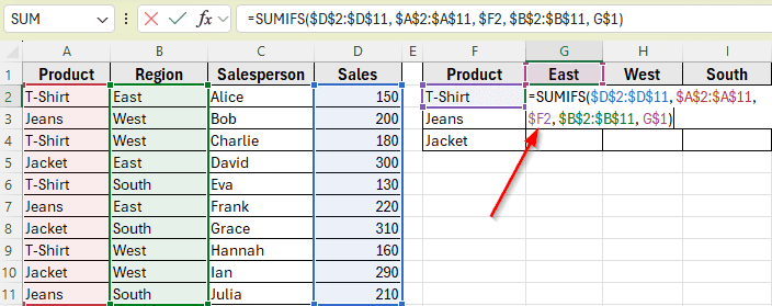
➤ Press Enter. The result will show the total sales for T-Shirt in the East region.
The dollar signs lock the ranges and headers so the formula updates correctly when copied across the table.
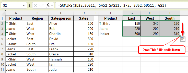
➤ Now drag the formula to the right for other regions like West and South.
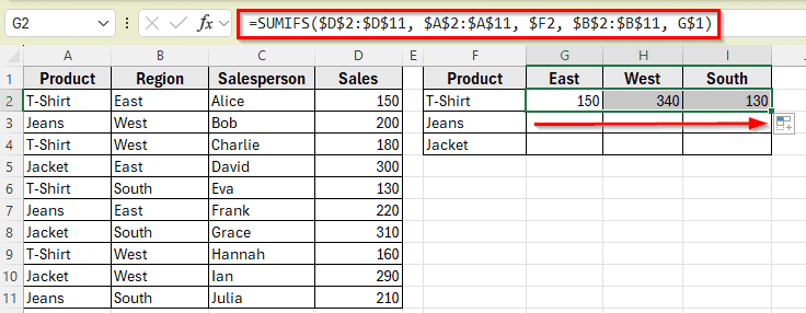
➤ Then drag the entire row down for other products like Jeans and Jacket.
Apply SUMIF Function With a Combined Condition
The SUMIF function in Excel is built for one condition only. If you want to sum values based on two criteria, like where Product is T-Shirt and Region is East, you’ll need a workaround. One way is to use a combination of SUMIF functions to simulate multiple conditions.
To sum sales where the Product is T-Shirt and Region is East, we can first create a helper column that combines both conditions into one text string.
Step 1: Add a Helper Column
➤ Open your dataset in Excel. First, we’ve to add a helper column in Column F. For example, select cell F2.
➤ In cell F2, insert a formula that combines Product and Region:
=A2 & “-” & B2
➤ Now the row will look like T-Shirt-East.
➤ Drag down the formula to the rest of the rows. For example, cell F2 to F11.

Step 2: Use SUMIF on the Combined Column
➤ Now, type this formula in cell G2
=SUMIF($F$2:$F$11, F2, $D$2:$D$11)
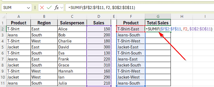
➤ Press Enter. You’ll see the result of total sale in cell G2, which is 150.
➤ Drag the formula across the matrix to fill other cells. Each result in Column G will now show the total sales for the corresponding Product–Region combination listed in Column F.

Drawback of Using SUMIF Function
When you use the SUMIF function with a helper column, you need to make sure that each item in your summary list appears only once. If a Product–Region pair is repeated, the total will also repeat, like “T-Shirt-West” showing the same result twice in the image.
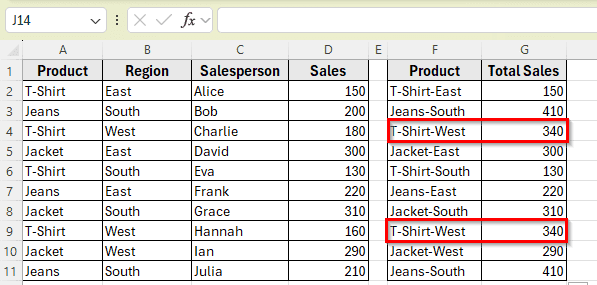
To fix this, keep your summary list clean by removing any duplicates before applying the formula.
Alternative to SUMIF: SUMPRODUCT for More Control
If you want more flexibility when working with multiple criteria, the SUMPRODUCT function is a powerful alternative to SUMIFS. It allows you to create custom logic by multiplying arrays of conditions and works well when you need more advanced calculations.
In this method, we’ll use SUMPRODUCT to calculate the total sales based on both Product and Region, like we did with the SUMIFS function. But instead of relying on fixed condition ranges, we’ll use a formula that evaluates each row using logical checks.
Here’s how to apply this method:
➤ Open your dataset in Excel.
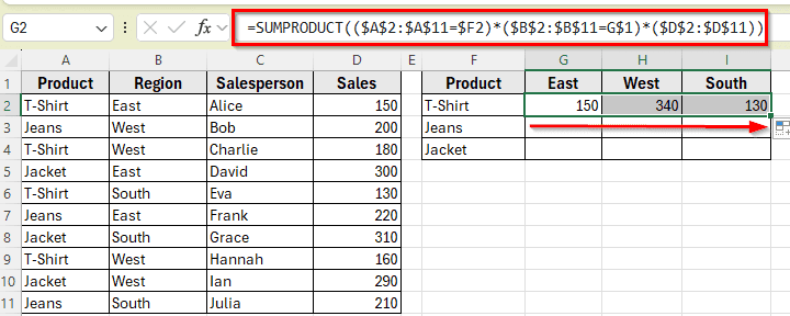
➤ Click on cell G2, where you want to calculate the total sale for T-Shirts in the East region.
➤ Type the following formula
=SUMPRODUCT(($A$2:$A$11=$F2)*($B$2:$B$11=G$1)*($D$2:$D$11))
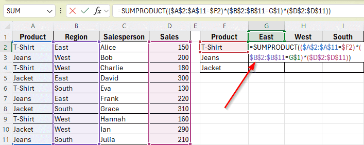
➤ Press Enter.
➤ The result will show the total sales for T-Shirts in the East region.
Each condition returns an array of TRUE or FALSE values, which are treated as 1 or 0. The formula multiplies the condition arrays together with the sales values and adds up only the matching rows.
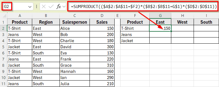
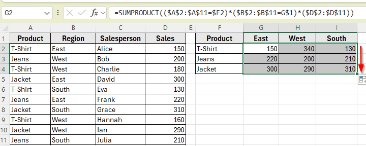
➤ Now drag the formula across to fill the West and South columns.
➤ Then drag the row down to calculate totals for Jeans and Jacket as well.
➤ Each cell will return the correct total based on the matching Product and Region.
Frequently Asked Questions
How do you use SUMIF with multiple criteria in different columns?
The SUMIF function only works with one condition. To apply multiple criteria across different columns, use SUMIFS instead. It lets you apply more than one condition to filter your data.
How to use SUMIFS with multiple criteria in different columns in Excel?
To use SUMIFS function with multiple criteria in different columns, you can pass each condition along with its corresponding range. For example, if you want to sum the values in Column D when the Product in Column A is T-Shirts and the Region in Column B is East, use this formula:
=SUMIFS(D2:D11, A2:A11, “T-Shirt”, B2:B11, “West”)
This formula checks both conditions row by row and adds only the sales values that match both.
Wrapping Up
Summing data based on more than one condition across different columns is useful when you’re analyzing sales, tracking performance by category, or building summaries from large datasets. Excel provides several ways to do this effectively.
The SUMIFS function is the most used and simple option. It lets you apply multiple filters across separate columns and returns accurate totals. It’s especially helpful in matrix layouts, where you want to break down results by row and column criteria.
For more flexibility, the SUMPRODUCT function allows custom logic using arrays and conditions. And if you’re working with SUMIF, you can still handle multiple criteria by combining values in a helper column.
Each method helps you automate your calculations and reduce manual work. Pick the one that fits your task and use it to make your Excel reports more dynamic and reliable.