Performing a lookup from multiple columns and returning a value based on a matching result in Excel is a common yet advanced task. It is especially useful for analyzing complex datasets, managing cross-referenced information, or validating data entries. There are many built-in tools in Excel that allow users to perform this complex operation.
Follow the steps below to use VLOOKUP function for multiple columns with only one return:
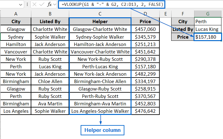
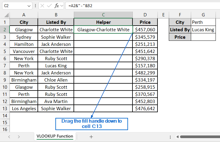
➤ In the dataset, create a new Helper column by concatenating the values in columns A and B using the formula:
=A2&”-“&B2
➤ Then, go to the lookup section of your worksheet and return the corresponding value by putting the formula:
=VLOOKUP(G1 & “-” & G2, C2:D13, 2, FALSE)
In this article, we will learn three easy and effective methods of using VLOOKUP from multiple columns with only one return.
Use VLOOKUP Function with Helper Column
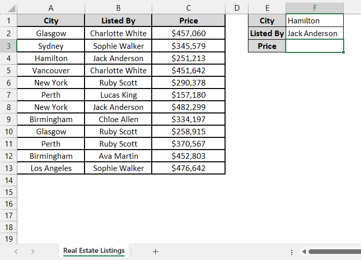
In the sample dataset, we have a worksheet called Real Estate Listings containing information about City, Listed by and Price. By using the VLOOKUP function, we will return a value in the Price cell based on the values entered in the City and Listed By cells. We will display the updated dataset in a separate worksheet called VLOOKUP Function.
The VLOOKUP in Excel is a useful function that searches for a value in the first column of a range and returns a corresponding value from another column in the same row. In this method, we will use a helper column to return a single value from multiple columns using the VLOOKUP function.
Steps:
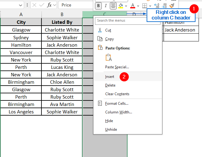
➤ Open the VLOOKUP Function worksheet, create a new column by right-clicking on the header of column C and selecting Insert from the context menu.
➤ Rename the new column as Helper, and in cell C2, put the following formula:
=A2&”-“&B2
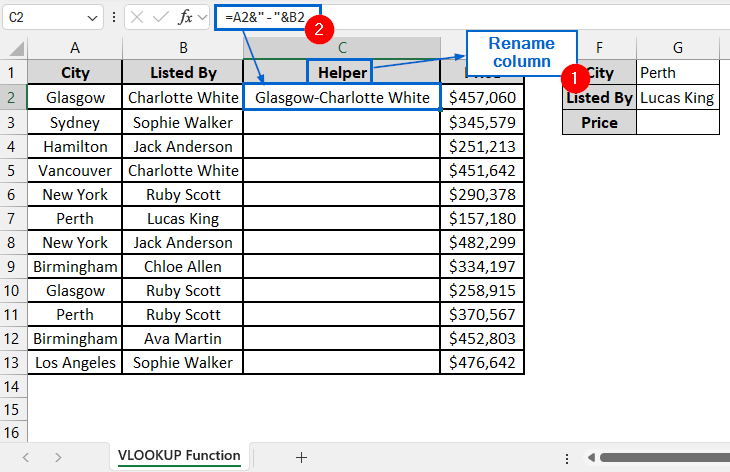
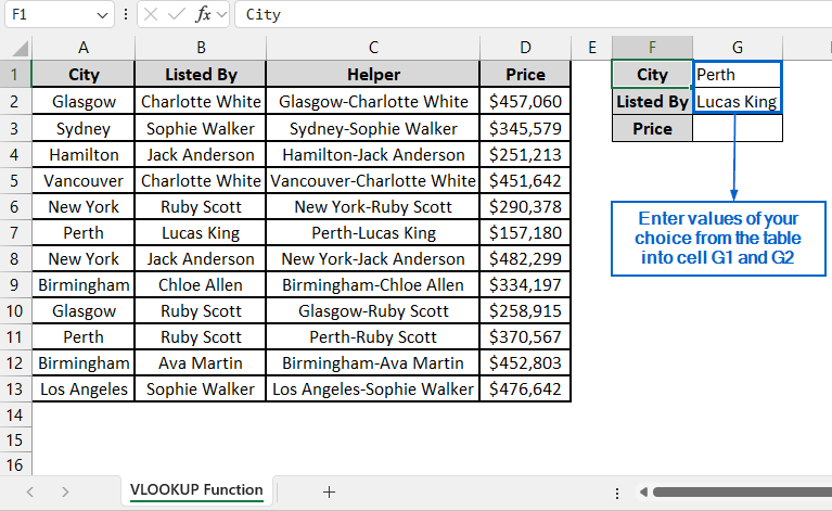
➤ Next, select cell C2 again and drag down the fill handle to apply the formula across the entire column.
➤ Now, enter a value of your choice from the table in cells G1 and G2.
➤ After entering the value, select cell G3 and put the formula:
=VLOOKUP(G1 & “-” & G2, C2:D13, 2, FALSE)
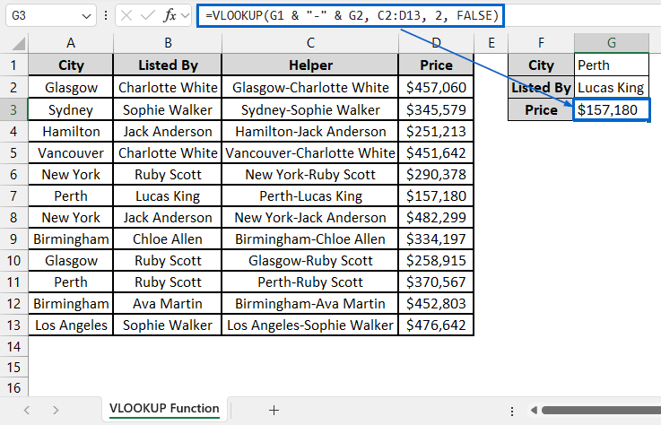
➧ G1 & "-" & G2 is used to join the values in cells G1 and G2 into a single string.
➧ C2:D13 is the lookup range that the formula uses to return the corresponding Price from column D, based on the combined Helper value in column C.
➧ “2” tells the formula to return the value from the second column in the range (column D).
➧ FALSE ensures that the formula returns an exact match only.
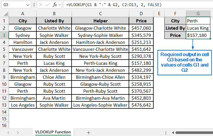
➤ You should now have the required value in cell G3 based on the corresponding values entered in cells G1 and G2.
Insert XLOOKUP Function to Return a Value Directly
The XLOOKUP function in Excel is another useful tool that allows users to search a range or array for a specific value and return a corresponding value from another range. Unlike the previous method, we do not need any helper column to return a value.
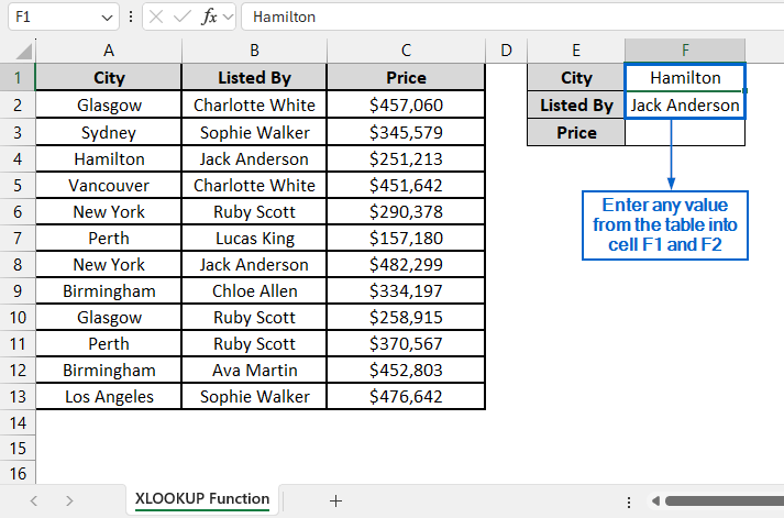
Working with the same dataset, we will return a value in cell F3 based on the values put in cells F1 and F2. The updated dataset will be stored in a separate worksheet called XLOOKUP Function.
Steps:
➤ Open the XLOOKUP Function worksheet and put values of your choice from the table in City (cell F1) and Listed By (cell F2).
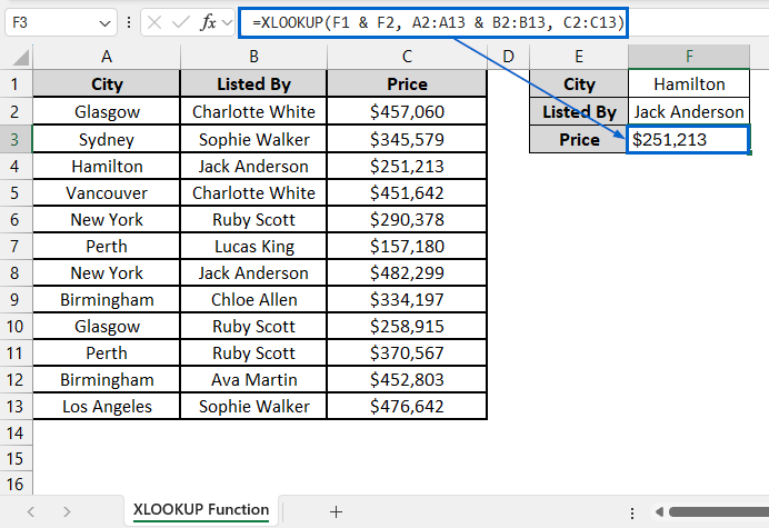
➤ Next, select cell F3 and put the formula,
=XLOOKUP(F1 & F2, A2:A13 & B2:B13, C2:C13)
➧ F1 & F2 joins the values in cell F1 and F2 into a single lookup value.
➧ A2:A13 & B2:B13 is used to concatenate the values in columns A and B for each row from 2 to 13, creating a combined text.
➧ C2:C13 is the return array from which the matching value will be retrieved.
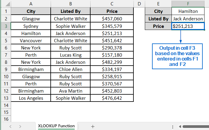
➤ Cell F3 should now return the matching value based on the data entered in cells F1 and F2.
Return a Single Value with INDEX-MATCH Formula
This is an advanced method in which we will use both the INDEX and MATCH functions to search across multiple columns and return a corresponding value based on specific criteria.
The INDEX function in Excel is used to return the value of a cell based on a specified row and column number within a given range. Whereas the MATCH function is used to find the position of a specified value within a range of cells.
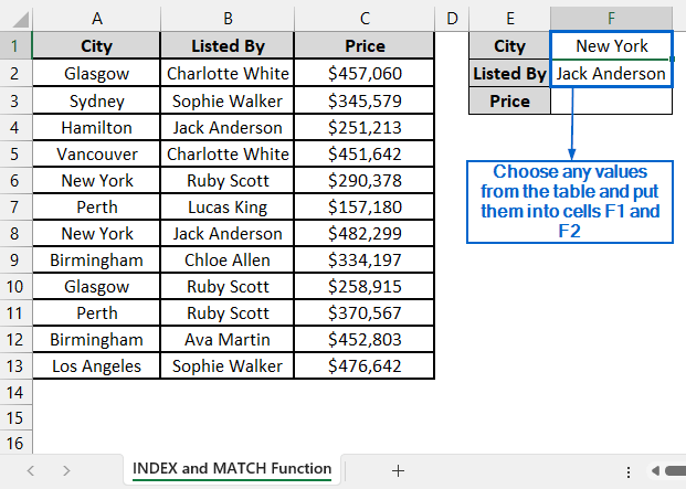
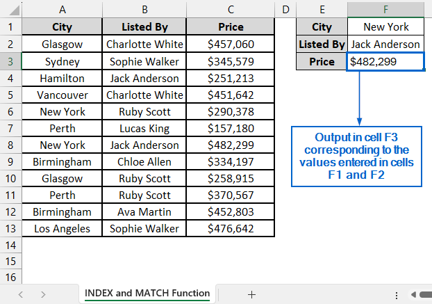
We will again work with the same dataset and use both INDEX and MATCH functions to retrieve the value in cell F3 based on the inputs in cells F1 and F2. The modified dataset will be stored in a separate INDEX and MATCH Functions worksheet.
Steps:
➤ Open the INDEX and MATCH Functions worksheet and enter any values from the table into cells F1 and F2.
➤ Next, select cell F3 and put the formula:
=INDEX(C2:C13, MATCH(1, (A2:A13=F1)*(B2:B13=F2), 0))
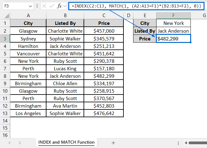
➧ (A2:A13=F1)*(B2:B13=F2) part creates an array where each row returns 1 if both conditions match, otherwise it returns 0.
➧ MATCH(1, ..., 0) is used to find the position of the first row where both criteria are met.
➧INDEX(C2:C13, …) part returns the value from column C at the matched row.
➤ The values corresponding to the entries in cells F1 and F2 should now be displayed in cell F3.
Frequently Asked Questions
Which Method is Best Suited For Large Datasets?
If you are working with large datasets, the INDEX and MATCH functions would be the most suitable. Unlike other methods, INDEX and MATCH functions do not create temporary combined arrays, which helps them run faster and use less memory.
Why is My Formula Returning #N/A Error?
If your formula is returning a #N/A error, it typically means that no exact match was found for the lookup value. Double-check your input values and make sure that the lookup ranges and criteria are correct.
Concluding Words
Knowing how to perform VLOOKUP in Excel from multiple columns with a single return value is important for managing datasets and streamlining workflows. In this article, we have discussed three effective methods of performing VLOOKUP from multiple columns with a single return, including using the VLOOKUP Function, XLOOKUP Function and combining INDEX with MATCH Function. Feel free to try each method and select one that best fits your needs.